
One-dimensional chain of quantum molecule motors as a mathematical physics model for muscle fibers
[Si Tie-Yan†a), b)  ]
]
]
|
|


†Corresponding author. E-mail: tieyansi@foxmail.com
*Project supported by the Fundamental Research Foundation for the Central Universities of China.
A quantum chain model of multiple molecule motors is proposed as a mathematical physics theory for the microscopic modeling of classical force-velocity relation and tension transients in muscle fibers. The proposed model was a quantum many-particle Hamiltonian to predict the force-velocity relation for the slow release of muscle fibers, which has not yet been empirically defined and was much more complicated than the hyperbolic relationships. Using the same Hamiltonian model, a mathematical force-velocity relationship was proposed to explain the tension observed when the muscle was stimulated with an alternative electric current. The discrepancy between input electric frequency and the muscle oscillation frequency could be explained physically by the Doppler effect in this quantum chain model. Further more, quantum physics phenomena were applied to explore the tension time course of cardiac muscle and insect flight muscle. Most of the experimental tension transient curves were found to correspond to the theoretical output of quantum two- and three-level models. Mathematical modeling electric stimulus as photons exciting a quantum three-level particle reproduced most of the tension transient curves of water bug Lethocerus maximus.
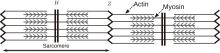
Muscles are comprised of bundles of cylindrical muscle fibers. One muscle fiber contains hundreds of thinner cylindrical fibers called fibrils. A fibril is a train of sarcomeres connected from head to tail. The sarcomere, as observed by light microscopy, is a composite structure of actin filaments and myosin filaments (Fig. 1). These two filaments are bridged by long myosin proteins called myosin molecule motors (see Refs. [1] and [2] or a biology textbook for a more detailed review).
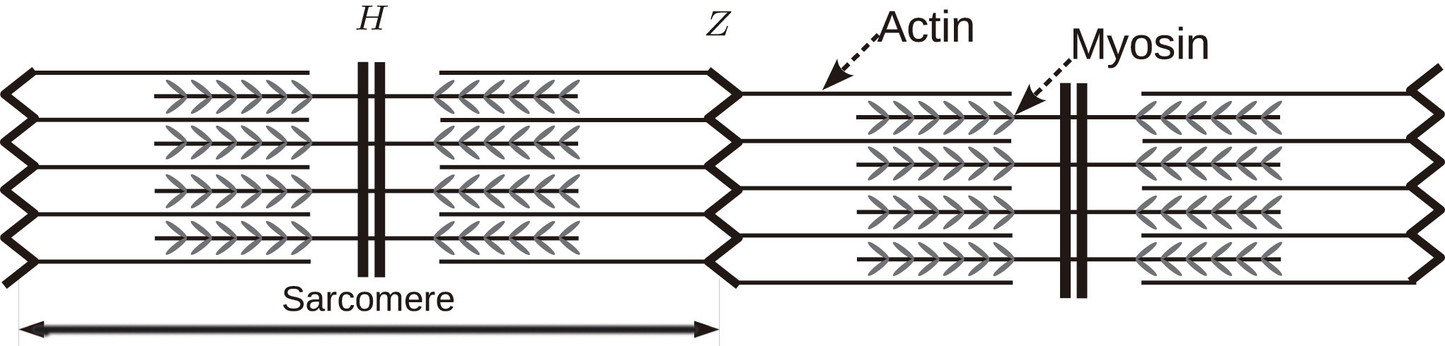 | Fig. 1. Longitudinal section of a filament array in muscle fibers. Myosin molecules are long polymers that act as cross-bridges between actin filaments and myosin filaments. |
The length of a sarcomere decreases during muscle contraction. Huxley modeled muscle contractions as mutual movement between actin filaments and myosin filaments.[3] When the myosin molecule in the myosin filaments is excited, attaching to the actin filament, a myosin molecule will combine with adenosine triphosphate, and convert energy from adenosine triphosphate hydrolysis into mechanical force — this is the attached state. In the detached state, the myosin molecule is at rest and does not function. The arrangement of myosin molecules along the length of the filament is variable. A stochastic model was introduced to describe these co-operative behaviors of molecular motors which have a disordered arrangement along the backbone.[4] Experimental research has progressed beyond the description of the classical mechanics two-state cross-bridge model[5] which assumed the probability of the two states, i.e., the detached state and the attached state, satisfy a pair of coupled differential equations.
Myosin molecules resemble long arms ending with a head domain. The myosin in muscle cells is usually called myosin-II, owing to its two heavy chains in the head domain. A second type of myosin molecule with a single heavy chain has been found in non-muscle cells, this molecule is called myosin-I. The average length of myosin-II is about 160 nm.[2] Visible light corresponds to a wavelength range of 400 nm– 700 nm. The electromagnetic wavelength comparable to the length of myosin-II falls in the ultraviolet region.
Muscle fibers are surrounded by membranes, which are under the control of nerve cells. The membrane acts as a filter system that is permeable to certain ions but impermeable for other ions. The imbalance in ions across the membrane results in an electric potential difference between – 60 mV and – 90 mV. The electric signals from nerve cells can modify the permeability of the membrane. An active muscle will generate an electric signal. Scientists can use this electric signal as a measure of the tension inside the muscle. If we insert a needle with two fine-wire electrodes into the muscle, the electric activity of the muscle can be detected and recorded by an oscilloscope. Such electromyograms are widely used for medical examinations of muscles.
Electromagnetic waves are called photons in quantum mechanics. The electric signal generated by active muscle is physically equivalent to a wave packet of photons. Quantum scattering between photons and molecules within a biological system is a common phenomenon and has been shown to occur in muscle. Molecules only absorb photons at resonance frequency. Therefore there must be a one-to-one correspondence between conformational changes in motor molecules and the transition between quantum states of a molecule. The excited quantum level can be defined as the attached states in which the motor molecule was extended to a longer shape. The detached state was assumed to be equivalent to a quantum state with a lower energy. The motor molecule becomes shorter in the detached state. In addition to the two quantum states of molecules, another quantum state of photons is thought to induce the transition between the two quantum level. Photons can propagate among different molecules. Such photons couple different motor molecules to work together. Quantum physics has many techniques to control quantum states, thus it is possible to control the conformation of molecule motors using electromagnetic waves.
Muscle fibers can also be stimulated by chemical solutions characterized by complicated biochemistry.[2] Although a prior study described chemical reactions in muscles using quantum mechanics, [6] this model is different from the model proposed in this text. Specifically, the time scale in the current model is much larger than the chemical reaction. Here I have focused only on the electrical stimulation of muscle fibers without adding any external chemical solutions. To make this mathematical physics model work in a real muscle fiber system, the following assumptions were necessary. First, the strength of electric field should be so strong that it dominates the conformation of molecules over thermodynamic fluctuations. Second, for muscle fibers not exposed to external stimulation by chemical ions, the conformational change in motor molecules governed by the electromagnetic field is much larger than that induced by chemistry. This is because the electric field is distributed across the whole space and it exerts a global force on the motor molecules. While chemical ions only interact with molecules locally, they do not function unless they find the correct binding site. Finally, the spatial conformation of motor molecules can be modified by concentration of some chemical ions.
In this text, muscle fibers have been simplified into a one dimensional chain of many giant quantum particles which represent molecule motors. The velocity of a sliding actin filament acts as an environmental parameter. These giant quantum particles are excited by absorbing photons and relaxed by emitting photons. In the proposed model, these particles were arranged regularly along a one-dimensional chain. The wavelength of the stimulus electromagnetic pulse was assumed to be much larger than a sarcomere. The configuration of spatial arrangement within a sarcomere was expected to have no influence on the output physics.
This article is organized as follows:
In Section 2, the quantum Hamiltonian for deriving analogous force– velocity relationships with respect to the corresponding macroscopic quantity is described. The empirical Hill’ s relationship is consistent with the steady solution of Heisenberg equations. The force– velocity relationships for slow release cases and the non-steady-state solutions were predicted. In Section 3, the mechanism through which the force decays after stimulation with an electric pulse is examined. The exact solution of a quantum two-level model reproduced similar tension activation curves in cardiac muscle. The analytical solution of a quantum three-level model could generate most similar curves of tension transients for insect flight muscle. In Section 4, the tension transient curve of skeletal muscle is mathematically in the context of quantum coherent state. The experiment curve coincided with the third-order projection of the coherent state. In Section 5, the self-coupled quantum Hamiltonian for solving strongly coupled differential equations is derived. For this case, the sliding velocity depended on the internal states of the motor molecule. The last section provides a brief summary and outlook.
In muscle release experiments, the two ends of the muscle are fixed at the resting length. Electric pulses with different frequencies are superimposed to develop tension in the muscle. In quick release experiments, one end of the muscle is set free quickly. For slow release experiments, the length of the muscle is shortened with one end of the muscle oscillating or moving under specific control within a relatively longer time interval. The tension– velocity relationship is the relationship between two macroscopic quantities. In the following text, the force is expressed as a microscopic density operator, while the velocity is considered a macroscopic parameter. The velocity of contraction was assumed to be controlled by the density of some ions in the solution. Only the excitation and decay processes of muscle were modeled.
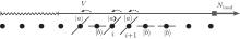
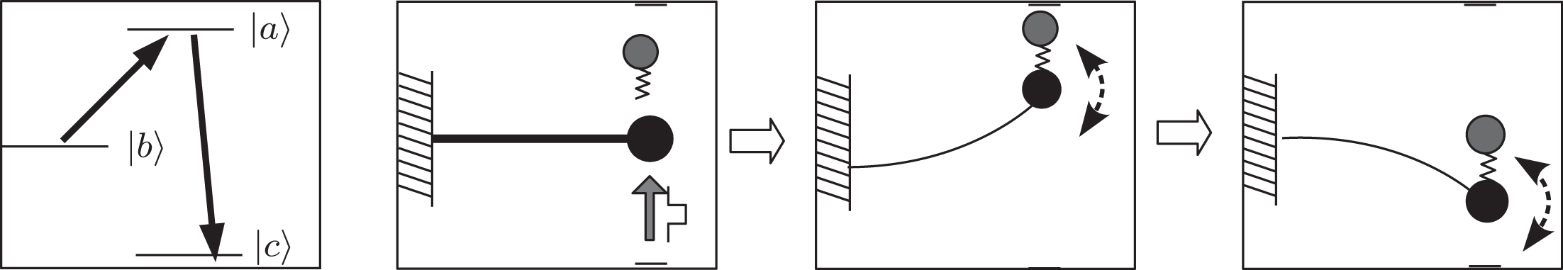
The myosin molecule motor could be characterized as a multi-level quantum particle. One eigenstate of the particle with respect to each level represents one conformation. In the excited state | a⟩ , a myosin molecule is attached to the actin filament. In the ground state | b⟩ , the quantum particle is at rest in the myosin filament. One photon may excite the quantum particle from the ground state to the excited state. The particle hops from state | a⟩ to state | b⟩ by emitting one photon. The quantum representation of the mutual sliding movement between the actin filament and myosin filament is characterized by elimination of one quantum state on one lattice site and generation of the same quantum states at the next nearest neighboring lattice site. Because the sliding motion has only one direction, switching two neighboring lattice sites would result in a negative hopping operator. The quantum Hamiltonian of this one-dimensional chain (Fig. 2) is unitary,

where s is the unit lattice spacing, and v is the absolute sliding velocity. The hopping coefficient gab(t) = p0E(t) is the electric field. The symmetric coupling coefficients gab(t) = gba(t) = g were usually chosen. This Hamiltonian was neither single-particle Hamiltonian nor a tight-binding model. For the particle at lattice site i, the probability of being in the excited level | a⟩ i was measured by the density operator, 


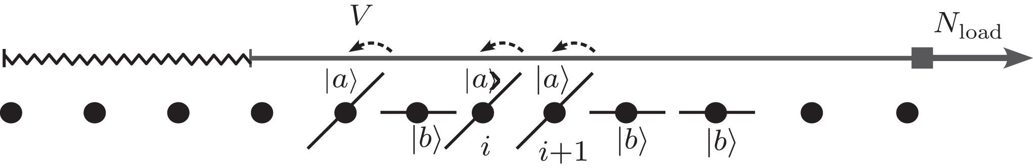 | Fig. 2. A one-dimensional chain of quantum two-level particles. Each particle represents one myosin molecule motor. |
The time evolution of the density operators were governed by the equation of motion, 
where 


where R(v) is the complicated function of velocity,
where k = ω /c, c is the speed of light. fn is the frequency of the stimulatory electric pulses, and Nt is the total number of particles. The tension of the one-dimensional chain was defined as the total number of particles in the excited state,

where χ is a renormalization coefficient, set as χ = 1 for convenience. In excited state, myosin is attached to the actin filament. As an increasing number of myosin molecules are excited, the physical bonds between the actin filaments and myosin filament become stronger. The maximal tension was determined by the total number of particles, Tensionmax = Nt, i.e., all particles are excited to connect the two filaments.
The existence of a maximal tension value was consistent with experiment measurements. If one applies a single electric shock across the membrane, the tension of the muscle fiber first increases from zero to a transient maximal point and then decays to zero. The electric shock is an energy packet with a finite number of photons. Suppose the energy packet contains Np photons, and Np < Nt. This would allow for maximum excitation of Np molecular motors. Additionally, the motor would be actively decaying and emitting photons. If Nt photons are sent into the muscle at one time before any decay process, all the molecules will be excited, and the muscle will reach the maximal tension state. A certain amount of time is always required for the muscle to consume all the photons, and more photons must be added to account for filling the loss of photons by decay.
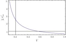
The relationship between the total probability density and velocity obtained for the steady state, i.e., Eq. (4), was found to be quite similar to Hill’ s empirical force– velocity relationship.[7] In the case presented here, the physical origin of every parameter was known. Although the complex function R(v) was included in Eq. (4), the tension– velocity curve exhibited a hyperbolic shape, and the tension decreased with increased velocity (Fig. 3). The equations of motion, i.e., Eq. (2) and Eq. (3), suggested that the velocity was actually a decay coefficient. Thus, greater velocity would lead to more rapid decay, and the number of physical bonds connecting the two filaments would decrease as the velocity increased. This result provided a natural explanation for the experimental results.
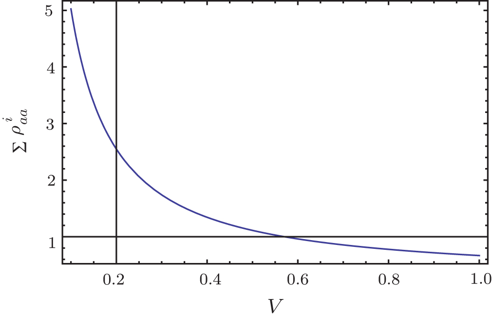 | Fig. 3. Numerical plot of the tension– velocity relationship according to Eq. (4). |
In addition to the decay induced by mutual sliding movement, spontaneous decay due to thermal fluctuation and vacuum fluctuation has also been observed. When considering spontaneous decay, the equation of motion for the density operator is given by

where Γ is the friction tensor, Γ i j = γ iδ i j. This equation of motion was similar to that of quick release,


where 

For the steady state, 
where 
If the velocity term is much larger than the spontaneous decay term, i.e., 2v/s ≫ γ a, γ b, one ignores spontaneous decay, and equation (11) is then reduced to the former tension– velocity relationship described by Eq. (4). Therefore, equation (4) defines the force– velocity relationship for the quick release of muscle. If the muscle is released slowly, the spontaneous decay may become as important as the velocity term, 2v/s ≈ γ a, γ b. In that case, the tension– velocity relationship should obey Eq. (11). Thus equation (11) is the general force– velocity relationships for steady state. For non-steady state conditions, it is necessary to solve the equations of motion to determine how the excited state density operator evolves as a function of velocity.
The insect flight muscle oscillates far more rapidly than the frequency of the input nervous impulse. A muscle is unable to expand, it only contracts. Muscle expansion is achieved by contracting an opposing muscle. The oscillation frequency of muscle is the frequency of the oscillation between the excited state and relaxed state. The 
was performed and equation (13) was then substituted into Hamiltonian Eq. (1). The Hamiltonian equation could now be written more briefly as,

where H0 is the exactly solvable part for the regulated free oscillator,
The regulated oscillation frequency depends on the velocity and momentum vector k. The free oscillation has a maximal frequency and a minimum frequency,
The band width for the existing free oscillation model is determined by the sliding velocity. An oscillating electric field,

would induce the hopping between two levels. The state vector for the Schrö dinger wave equation,

is written as

The density operator is given by 

where Δ ω = ω a – ω b. The non-steady state tension decreased following v– 2 regulated by an oscillation factor. The ultimate oscillation frequency of the tension includes three sources,

When the frequency difference of the two level vanishes, Δ ω = 0, the output frequency is utterly dependent on the sum of perturbation frequency and sliding velocity. The fast oscillating ion flow of K+ and Na+ across the membrane causes the potential to increase to + 40 mV and restores its original value within a few milliseconds.[2] This oscillation frequency coincides with some muscle oscillations. Some insect flight muscles contract 1000 times per second. Thus I hypothesize that the output oscillation frequency of muscle has some possible relationships with the oscillation of ion flow. Certain insect flight muscles can oscillate more rapidly than the frequency of the input nervous impulse. Equation (20) indicated that the output frequency depends not only on the frequency of the input nervous impulse, but also on the sliding velocity and the frequency difference between the two levels. The sliding velocity may increase the output oscillation frequency. The output tension measured in the experiment is the superposition of different oscillator modes,

The two ends of the one dimensional muscle fiber are always attached to some tissues. If there are N + 1 particles along the chain, the first and last particles are fixed. Because sin(ks) in dispersion Eq. (20) is a periodical function, the independent standing wave modes is confined in the domain (– π < ks < π ). The allowed wave modes are

where L is the length of one sarcomere. All particles are oscillating in a standing wave pattern with frequency ω . For selected modes mπ /L, the phase difference between the nearest neighboring particles is (mπ /L)s. If the sliding velocity is zero (v = 0), the standing wave mode is eliminated.
Stretch activation involves lengthening of the muscle fiber by an external force, or to release the fibers to certain length within an extremely short period of time. The fibers are glued between two glass rods, and one rod is attached to the anode pin of a force transducer. The length and tension signals are displayed on a double beam oscilloscope.[8]
Both the myosin filament and actin filament are long helical chains. The basic structure of a myosin filament resembles a golf club, and the filaments are entwined to produce a helix with a diameter of about 15 nm. Actin filaments have a double helix structure composed of globular protein. The local electric charge distributions along the myosin chain and actin chain are not homogeneous. Mutual sliding between the myosin and actin chains would inevitably modify the local potential configuration. Increasing or decreasing the local potential barrier would induce the transfer of electrons among different energy levels. Many photons are generated within a very short time. Stretch activation by mutual sliding movement is equivalent to stimulating the muscle fiber with an electric shock pulse.
The time evolution of tension induced by stretch activation includes two periods. In the first period, rapid decay occurs due to the extremely large sliding velocity. A large number of photons are generated but are not absorbed by the molecular motors. In the second period, the two filaments stopped their mutual sliding, and the accumulated photons began to play a role. This period is dominated by the spontaneous emission and absorption of photons.
The ideal definition for contraction velocity is

where L is the length of the sarcomere. In fact, the experiment measured the average velocity within Δ t. At the moment of quick release, the length experienced a sudden change,

The sliding velocity at t0 is almost infinity, v(t0) ≈ ∞ . However after the stretch, the length does not change anymore, and the sliding velocity becomes zero. The Heaviside function provides a good mathematical description for the variation in length during a stretch.
In the microscopic phenomenon, stretch activation would induce a sudden change in the particle distribution on different energy levels. There was an optimal distribution that acts as the minimal point of a potential configuration. Any deviation from this optimal point was associated with a tendency to return to the optimum. The optimal particle distribution was shown to be different for different types of muscle fibers. The external load applied to the muscle was actually a high potential barrier. The particles were trapped in a local minimal point to counterbalance the external force. Because a muscle is only able to contract, the intrinsic potential without the external load was asymmetric.
The stretch activation of cardiac muscle has been extensively studied.[8] Various different species of vertebrates have been examined, including humming birds, frogs, Guinea pigs, rats, rabbits. The tension transients following length perturbation were recorded using a force transducer. At the instant of muscle lengthening, the force jumps up to the maximal force, followed by a drop to a temporary minimum. After several small oscillations, the force finally reaches a new maximum. The length of the muscle was kept constant for a few seconds and was then suddenly released to its original length. A sharp drop in force appeared immediately followed by a fast recovery. The force transients for stretch and release were the mirror-image of each other (Fig. 5. in Ref. [8]).
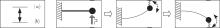
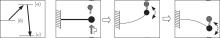
A quantum two-level system provides a good model for the physics of force transients of cardiac muscle. A mechanical analogy for this quantum model is an oscillator in thick liquid. As shown in Fig. 4, a heavy ball was attached to one end of an elastic rod. The sudden lengthening of muscle could be analogous to hitting the ball with a pulse. The ball would pop up to hit the upper level.
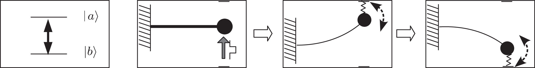 | Fig. 4. The mechanical oscillator as an analogy of the quantum two level model. |
Since the length of the muscle after the sudden stretch was maintained, a spring from the upper level could catch the ball to prevent it from returning to its original position. However, the elastic rod will pull the ball down, and the competition between the elastic rod and the spring from the upper level would induce local oscillations. When the kinetic energy was finally consumed by the friction of the thick liquid, the ball would stop oscillating. Analogous to the sudden release of muscle, a pulse hit the ball in the opposite direction of the lengthening. Because the molecular motor runs only in one direction, it is reasonable to introduce a bias potential. This bias potential makes it a little bit more difficult to restore the original position of the ball from the bottom level. Here the bias potential is the gravitational field.
It was assumed that the relaxed state of a muscle fiber was reached at the optimal ratio between attached states and detached states. One straightforward ratio was to set such that the numbers of particles in the excited state and ground state were equal. This relaxed state was the vacuum state of the quantum two-level model. This did not mean that there were no particles, but instead indicated that the number of particles was exactly the same as the number of antiparticles. In the mechanical analogy, this relaxed state corresponded to the equilibrium position of the ball without external pulses or the gravitation field. If a bias field existed, the mechanical equilibrium would be obtained by the balance between the gravitational field and the elastic force of the rod, κ Δ h = mgΔ h. We assumed that the optimal ratio was determined by the chemical potential of the two states,

where μ a and μ b are the chemical potential of the excited state and ground state, respectively. In the following discussion, the density matrix represented the difference between the usual density operator and the vacuum density operator. We simply denoted this as 
The lengthening activation of the muscle was equivalent to a positive pulse. All of the particles in state | b⟩ were driven to state | a⟩ .

The sudden release at t1 represented a negative pulse, and all particles shifted to state | b⟩ .

Thus the length perturbation provided the initial conditions for time evolution of the density operator. Because the length was constant after the stretch activation, the velocity term in Hamiltonian Eq. (1) could be ignored. The equation of motion, including spontaneous decay, was as follows:
where Δ ω = ω a – ω b. The coupling coefficient was chosen as the symmetric, gab = gba = g. The two degenerated states, i.e., Δ ω = 0, were the focus of this study. In the beginning, all particles were in state | b⟩ , ρ α β (0) = δ α bδ β b. This corresponded to a quick release. Applying the standard ansatz
one reduces the differential equation to an algebra equation.[9] This finally yields the time evolution of probability in state | a⟩ , [9]
This is the conventional solution in the textbook of quantum optics.[9] The plot of this solution for three different cases is also shown in the book of Ref. [9]. I will reproduce some of the figures from this textbook[9] to show the shape of the tension transient curve, and will compare different cases with experimental curves, for which I have not obtained the copyright to use here. ρ aa(t) governs the tension transient. Here

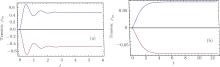
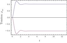
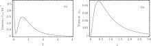
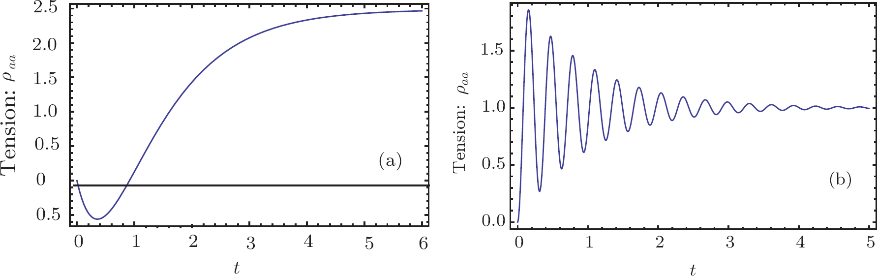
After stretch activation, there is no more external stimulus. The molecules undergo radiative damping through spontaneous emission. The time evolution of ρ aa(t) relies on the ratio between the driven field g and the damping rate γ , here we have set γ 1 = 2γ , γ 2 = γ . If the driven field is much larger than the damping field, there is an oscillation upon the exponential increase of tension (the upper curve in Fig. 5(a)). In the opposite case, the damping dominates the dynamic evolution and exhibits an exponential increasing without oscillation (the upper curve in Fig. 5(b)). Because the density operator must satisfy ρ bb + ρ aa = 1, the time evolution of ρ bb = 1 − ρ aa just follows the curve of ρ aa. For the intermediate case, the pumping strength is comparable to the damping rate, and both the lifetime and amplitude of oscillation are reduced as the pumping strength approaches an exponential increase for ρ aa(the upper curve in Fig. 6) or an exponential decay for ρ bb(the lower curve in Fig. 6).
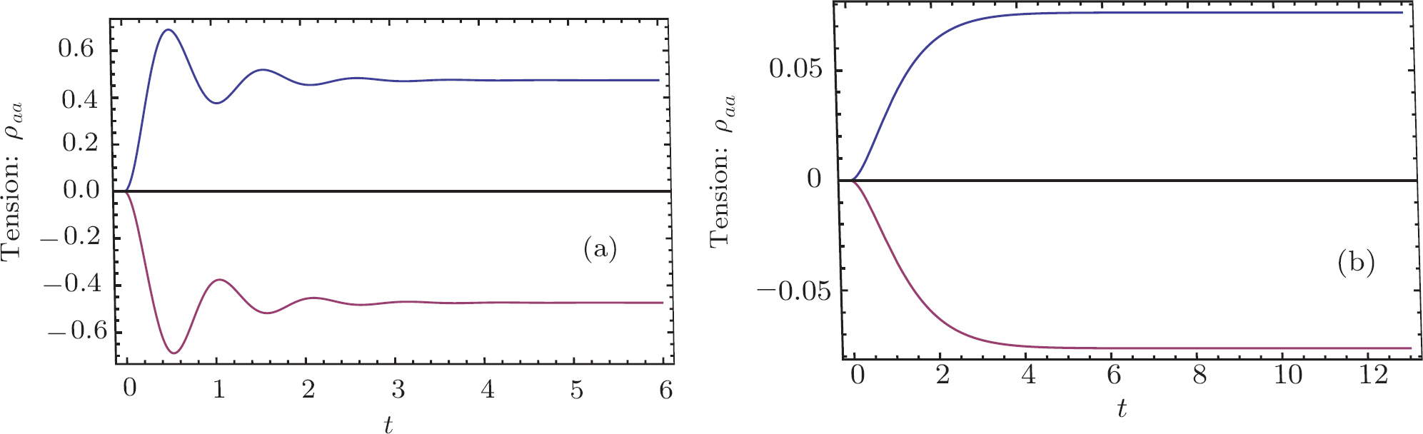 | Fig. 5. (a) The upper curve is the tension transient of ρ aa for a strong pumping field and low damping rate, g/γ = 3. The lower curve is the time evolution of (ρ bb − 1). (b) The tension transition for a weak pumping field and high damping rate, g/γ = 0.3. The upper curve is ρ aa(t), and the lower curve is (ρ bb − 1). |
 | Fig. 6. The time evolution of ρ aa(t) for g/γ = 1.5 (the upper curve). The lower curve is (ρ bb(t) − 1) for g/γ = 1.5. |
Comparing these tension transients curves with experiment records, [8] the data for ρ aa(t) in Fig. 5(a) fits well with the muscle tension transient under stretch activation, including the tension-time course of rabbit papillary muscle in Fig. 2 of Ref. [8], and the tension-time course of cardiac papillary muscle and insect flight muscle in Fig. 26 of Ref. [8]. In terms of the release activation, the tension-time courses of rabbit papillary muscle in Fig. 26. A of Ref. [8] and Fig. 2 of Ref. [8] fits very well with ρ aa(t) in the theoretical Fig. 6.
The tension-time courses of humming bird muscle under stretch activation and release activation were mirror images of each other, however, the life time and amplitude of tension oscillation under stretch activation were larger than that for the release case (Fig. 5 of Ref. [8]). The stretch activation curve fit well with ρ bb(t) − 1 in Fig. 5(a)). The release activation curve fit better with ρ aa(t) in Fig. 6. The release activation represented the tension recovery from state | b⟩ , whereas the stretch activation was the recovery from | a⟩ . The asymmetric tension-time course indicates the damping rate for | b⟩ was higher than the damping for state | a⟩ . In the mechanical analogical phenomenon, the damping may come from friction created by the liquid or the bias external field. In polymer physics, the extension process of a long polymer is not always exactly the reverse process of contraction. It is possible that the motor molecule may have a similar behavior, leading to the asymmetric tension time course. This can be called the hysteresis phenomena.
The tension-time course for a weak pumping field and high damping rate (Fig. 5(b)), g/γ = 0.3, reproduced the high tension state of rabbit psoas muscle. The tension transient of stretch and release was the mirror-image of exponential decay (Fig. 15A in Ref. [8]).
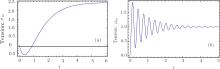
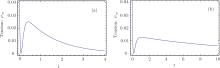
The tension transient Eq. (30) has two extremes. The first is for extremely high friction γ ≫ g, wherein the tension first decreases, and then exponentially increases to reach a stable value. The other case is for a very strong pumping field, g ≫ γ . In this case, the tension exhibits rapid oscillation, the envelope of the oscillation exhibits an exponential decay curve. These two cases are different from the previously described tension-time courses.[8] A mechanism may exist to prevent the cardiac muscle from falling into these two extreme cases.
 | Fig. 7. (a) The time evolution of ρ aa(t) for the case in which friction γ is much higher than the pumping field g, g/γ = 0.05. (b) The time evolution of ρ aa(t) for g/γ ≫ 1, the driving field is much higher than the friction. |
The tension transients of insect flight muscle under length perturbation were different from those of vertebrates including rabbits, humming birds, frogs, pigs, and so on. A previous study[8] reported the muscle tension course of the water bug Lethocerus Maximus. If the muscle is prepared in a regular solution without Ga+ + , the muscle tension is not highly responsive to length perturbation. However, in the presence of Ga+ + and Mg+ + , the significant tension transient of Lethocerus Maximus muscle can be observed in reaction to length perturbation.[8]
Under both stretch and release activation, the tension-time course curve showed a rapid rise to a transient maximum followed by a slow decay.[8] The shape of the decaying tail was beyond the theoretical prediction of the quantum two-level model. However, the quantum three-level model fit the experimental data very well. This suggested that the molecular motors in insect flight muscle may be different from the motors in cardiac muscle.
The insect flight muscle is still modeled as a one-dimensional chain of quantum molecule motors. However, in this model, the molecule motor has three states: the attached state | a⟩ , the metastable state | b⟩ and the detached state | c⟩ . The hopping between different states was assumed to be induced by vacuum fluctuation. Since muscle works at room temperature, the stochastic environmental fluctuation may destroy the coherent correlationships between different motors. The motors are almost independent from each other, thus the one particle model is a good approximation. The general Hamiltonian for a three-level particle interacting with vacuum modes reads,

where ω α β = ω α – ω β is the frequency difference between state | α ⟩ and | β ⟩ , α , β = a, b, c. dk and 


The quantum three-level system could be represented using a mechanical analogy similar to that of the damping oscillator for the two-level model. The key difference is that the oscillator has a metastable partner suspended above the equilibrium position (Fig. 8). To perform a lengthening perturbation, a shock pulse was sent to hit the oscillator in the opposite direction of gravitation. The oscillator would rise to attach to the partner ball, creating a pair. The pair would first rise to the attached state| a⟩ , and then decay to the detached state | c⟩ . For a sudden release perturbation, the shock pulse would hit the ball along the direction of the gravitation field. The oscillator first drops to the detached state | c⟩ , and is then pulled up by the elastic rod. The oscillator then continues to rise until it is high enough to attach to the metastable ball, and the ball and oscillator then oscillate as a pair. This damping oscillator model provides a general phenomenon to describe the tension– time course for insect flight muscle.
 | Fig. 8. The mechanical oscillator analogy of the quantum three level model. |
The myosin molecule motors is assumed to be an equivalent three-level system. The tension of the one-dimensional chain is proportional to the total number of particles in the attached state, Tension 

The molecule is initially in the attached state | a⟩ and metastable state | b⟩ . When the frequency difference between the attached state and metastable state is much smaller than the frequency difference between the attached state and detached state, i.e., ω ba ≪ ω bc, ω ac, the Schrö dinger equation admits an analytical solution, [10]
where the coefficients A and B are

The decay rate of the two upper levels are

D(ω ) is the mode density. λ 1, 2 determines the amplitude of the decaying metastable state,

where Δ γ = γ b − γ a is the difference in decay rates of the two upper levels. The probability of being in the attached state is given by the density operator ρ aa(t). Here the weights of the state vector, Ca(t) and Cb(t), define ρ aa(t) and ρ bb(t),

This density operator is actually a reduced density operator calculated by tracing out all of the vacuum modes,

To obtain a clear comparison with the two-level model, the Schrö dinger equations of motion for Cα [10] were mapped into the equations of the density operator,

The sum of the probabilities in the three levels satisfies the constraint, ρ aa + ρ bb + ρ cc = 1. For the two-level model, the sum of the probabilities in the two level is conserved, ∂ t [ρ aa + ρ bb] = 0. However, for the three-level model, ρ aa + ρ bb = 1 − ρ cc, the sum of the probabilities in the upper two levels depends on the probabilities in the detached state | c⟩ . The equations of motion (39) have already incorporated the evolution of ρ cc. One may verify ∂ t[ρ aa + ρ bb] ≠ 0 in Eq. (39).
The two excited states are coupled to the detached state by the same vacuum modes. The photon emitted by the transition from | b⟩ to | c⟩ may induce the transition from | c⟩ to | a⟩ . These photons may come from one molecule, but be absorbed by another molecule. Thus there is strong quantum coherence between the two-decay channel. A sudden lengthening in or release of muscle leads to mutual sliding between the charged filaments. A packet of photons is created immediately but is not absorbed. The stretch activation and release activation set up the initial value of population at a different level. The deviation from equilibrium position yields in a target potential barrier, which keeps a certain number of excited molecules from tunneling into a lower level. The number of surviving attached states determine the final tension value after decay.
One qualitative conjecture of Ref. [8] is that Mg+ + is able to vary the Ga+ + sensitivity of the contractile system. When the Lethocerus Maximus muscle is in a regular solution with only Ga+ + ions, the tension reaches the delayed maximum within 70 ms.[8] When Mg+ + is added, the time to reach the maximum tension becomes much longer, it is about 500 ms.[8] Figure 18B in Ref. [8] showed the tension time course in Ga+ + and Mg+ + contraction solution. The experiment was performed at a temperature of T = 18 ° C with 5-mM ATP. The ion concentrations were estimated to be pGa = 8 ∼ 9, pMg = 7 ∼ 8, pH = 6.5. Figure 23 in Ref. [8] shows a case in which the concentrations of Ga+ + and Mg+ + were even much higher than that for Fig. 18B in Ref. [8]. The tension– time course of Fig. 23 in Ref. [8] was recorded at temperature of T = 18.5 ° C with 5-mM ATP, pH = 6.5, pMg ∼ 5, and pGa ∼ 6.8.
I propose an analogous theoretical model in which the damping rate of the excited state is related to the relative ratio of Mg+ + to Ga+ + and the absolute values of their concentrations. Increasing Mg+ + may reduce the decay rate; that is, higher concentration may induce a lower decay rate. This theoretical conjecture is based on the solution of the three-level model in Eq. (34). Two very similar tension-time courses were found for the experimental curve in Fig. 18B in Ref. [8]. The first (Fig. 9(a)) simulates the stretch activation, for which the initial probability in the attached state is ρ aa(0) = 0.2. The second (Fig. 9(b)) is for the release activation. No particle exists initially in the attached state. To obtain tension transient curves similar to those in Fig. 23 in Ref. [8] from the three-level model, the value of damping rate γ a was raised from 4 to 14 in the numerical calculation. The theoretical output in Fig. 10 can be identified as the experimental curve of Fig. 23 in Ref. [8]. This theoretical curve in Fig. 10 showed a slower decay process compared with the two decay curves which were created in the context of lower concentrations of Mg+ + and Ga+ + (Fig. 9).
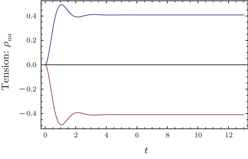
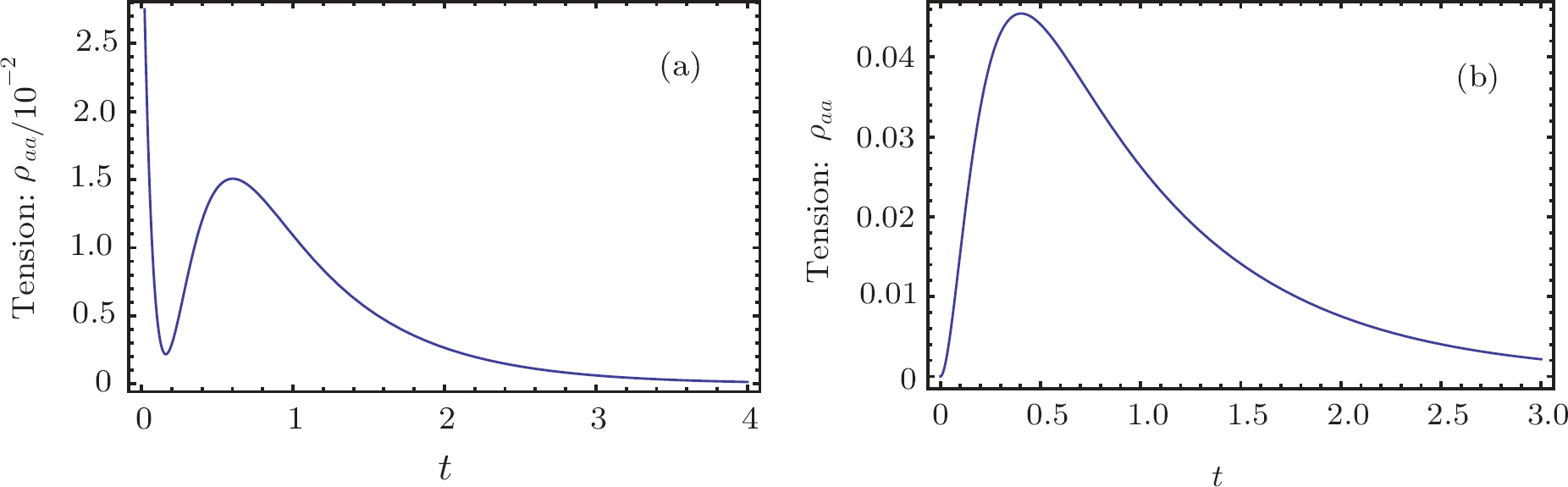 | Fig. 9. (a) The initial population in the metastable state is ρ bb(0) = 0.8. The attached state is ρ aa(0) = 0.2. The decay rate of metastable state is γ b = 7. The decay rate of the attached state is γ a = 4. The frequency difference of the two excited states is ω ba = 4. This curve corresponds to a stretch activation. (b) No population initially existed in the excited state ρ aa(0) = 0. ρ bb(0) = 0.5, γ b = 7, γ a = 7, ω ba = 4. This corresponds to a release-activation. |
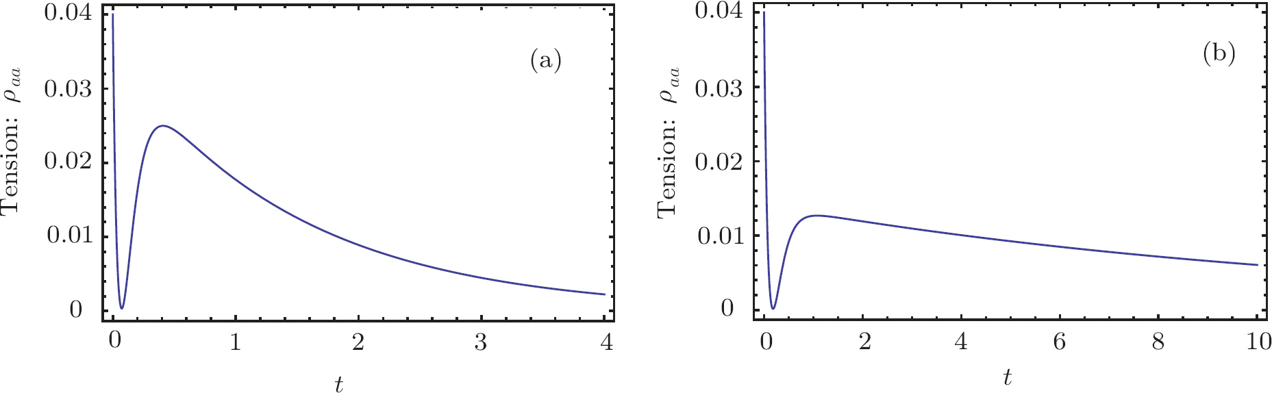 | Fig. 10. (a) Compared with Fig. 9, the decay rates for the attached state increased to γ a = 14. γ b = 7, ω ba = 4, ρ bb(0) = 0.5, ρ aa(0) = 0.2. The tension decay became slower. (b) The decay rate is γ a = 4. The frequency difference is reduced to ω ba = 1. γ b = 7, ρ bb(0) = 0.8, ρ aa(0) = 0.2. |
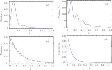
The frequency difference ω ba indicates the oscillation between the two excited states. The exponential decay of tension was strongly regulated by this oscillation. For small value of ω ba = 14, the tension had a dominant peak followed by small waves (Fig. 11(a)). If we magnify the tension course of experiment Fig. 19 in Ref. [8], the theoretical figure 11(a) would coincide with the experimental curve. This curve in Fig. 19 in Ref. [8] was obtained at a temperature = 23 ° C with 15-mM ATP, and at pGa = 8 ∼ 9. pMg = 7 ∼ 8, pH = 6.5. Comparing the current experimental condition with those for Fig. 18 in Ref. [8], it is clear that there was an increase in temperature by about 5 ° C and that the concentration of ATP was increased from 5 mM to 15 mM. Therefore, I hypothesized that increasing the concentration of ATP and the temperature could have enhanced the oscillation between the two excited states.
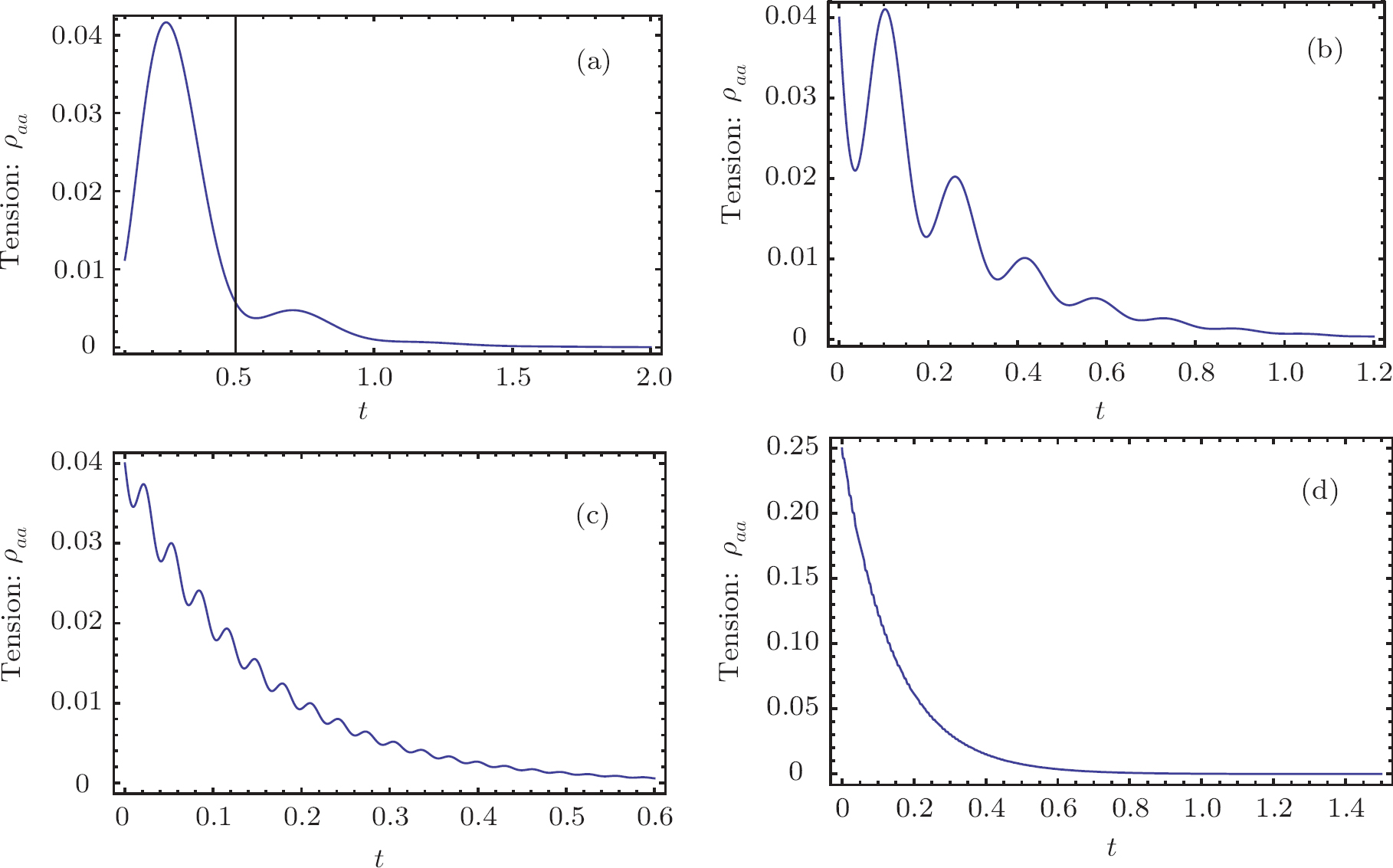 | Fig. 11. (a) The frequency difference between the metastable state and attached state ω ba is very large, ω ba = 14. ρ bb(0) = 0.8, ρ aa(0) = 0.2, γ b = 7, γ a = 4. (b) The frequency difference ω ba increases to ω ba = 40. ρ bb(0) = 0.8, ρ aa(0) = 0.2, γ b = 7, γ a = 4. (c) ω ba is ω ba = 200. ρ bb(0) = 0.5, ρ aa(0) = 0.2, γ b = 7, γ a = 7. (d) ω ba is almost infinity, ω ba = 900. ρ bb(0) = 0.5, ρ aa(0) = 0.5, γ b = 7, γ a = 7. |
If ω ba was increased, i.e., ω ba = 40, the decay process showed more frequent periods of oscillation (Fig. 11(b)). When ω ba = 200, the tension– time course became a wavy curve of exponential decay (Fig. 11(c)). This wavy curve was quite similar to the tension transient observed in rabbit psoas muscle (Fig. 15B in Ref. [8]). For an infinite large frequency difference, ω ba = 900, the oscillation was completely suppressed. The tension transients approached a smooth exponential decay (Fig. 11(d)), which resembled the experimental curves observed in the high tension state (Fig. 23C, in Ref. [8]). The high tension states of Lethocerus Maximus muscle are reached by increasing pGa from 8∼ 9 to 6.8, and maintaining pMg = 7 ∼ 8. From a theoretical point of view, a large frequency difference ω ba produced a large energy barrier. The quantum interference between the two excited states was no longer observed. Based on the theoretical approximation used here, ω ba ≪ ω bc and ω ba ≪ ω ac, a large ω ba indicated that the excited states were almost decoupled from the ground state. The dynamics of the three-level system were dominated by decay of the excited state. Since no pumping field could pass an infinite barrier, the evolution of the excited states was considered to proceed through exponential decay.
When the frequency difference ω ba was no longer presented, the two excited states became degenerated. Both of the states obeyed an exponential decay,
The tension could now be expressed as the sum of the probability of the two degenerated states, Tension = ρ aa(t) + ρ bb(t),

Thus, a tension evolution could be viewed as exponential decay plus a constant term. The maintenance of constant tension depended on the initial value of the density operator. For this special case, a three-level model with two degenerated excited states yielded results similar to those of the two-level model. However, the induced decay was always occurring owing to the emitting photons in the three-level model due to the metastable state. In the two-level model, the emitting photons could be brought back to the excited state without violating selection rules, thus the output of the two-level model did not produce all of the decay curves observed in the three-level model.
Compared with cardiac muscle and insect flight muscle, skeletal muscle has two special characters: low resting stiffness, and its ability to extend far beyond its optimal length. When these two special characteristics are applied to theoretical modeling, low stiffness indicates there are fewer molecular motors in the attached state when the muscle is not excited. Reducing bonding between two filaments allows for easier extension of fiber. The electrical signal representing muscle tension can be physically explained as polarized photons. The strength of the electric signal is proportional to the density of the photons. Quantum coherent photons exist in many living biological systems.[11] Even though an isolated muscle fiber is not alive, their data can still provide important insights into twitch tension evolution in reaction to an electric signal based on coherent states.
An external stimulus field will generate tension in the muscle. If the two ends of a muscle’ s fibers are fixed, the tension developed by the external stimulus is called isometric tension. The isometric tension of skeletal muscle was first measured many decades ago.[12] A supermaximal rectangular pulse is used to stimulate the muscle. Both the second and third derivatives of twitch tension are recorded using specialized software.[12]
Taking the same quantum Hamiltonian Eq. (14) of the one-dimensional chain of quantum two-level particles for modeling skeletal muscle,

The exactly solvable Hamiltonian H0 is given by Eq. (15). A quantized electric field induces transfer between the two levels,

where d is the annihilation operator of photons. Applying the conventional rotating wave approximation, the total Hamiltonian reads,

where

Hamiltonian Eq. (44) shares a very similar formulation with the general Hamiltonian for a coherent state.[13] If there is no special projection for a certain number of photons, a coherent state for photons would always be observed. However, one must project the coherent state to a fixed number of photons to obtain similar curves for the tension– time course of skeletal muscle. The off-diagonal density operator ρ ab was designated by a brief symbol ρ = (i/ħ )ρ ab. The Schrö dinger equation,

may be expressed by Fock states,
Here, the annihilation and creation rule of the photon operator in input is as follows:

Equation (47) is equivalent to a radioactive decay equation from which one can obtain the standard Poisson distribution.[14] Physicists define the coherent state as the eigenstate of the annihilation operator d. The coherent state with respect to Hamiltonian Eq. (44) is | ρ t⟩ ,

The general expression of a wave function as a solution of the Schrö dinger equation is

Projecting the coherent state | ρ t⟩ to the Fock space yields the Poisson distribution,

This coherent state is the superposition of many photon states. A photon is the electromagnetic radiation of quantum particles. Usually the electromagnetic radiation of human muscle is in the infrared region at a wavelength of tens of microns. For detection of electric signal in a muscle, a metallic needle is generally used. Therefore, the detector of the photons is assumed to have an optimal window that only allows a finite number of photons to pass, not all of the photons could be captured at one time. The projection of a coherent state with this optimal photon number state was measured in experiment. This electric signal is proportional to the amplitude of the optimal photon state,
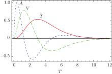
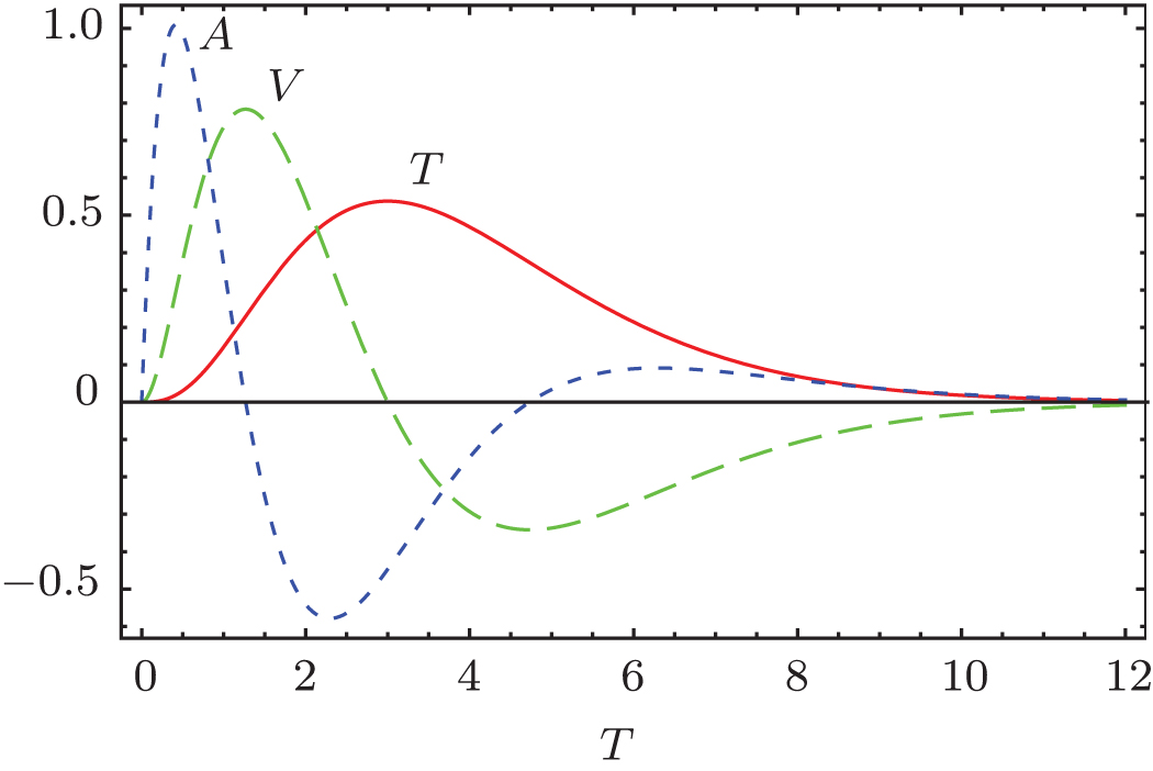
The experiment described in Ref. [12] only reported one complete tension– time course (Fig. 1E in Ref. [12]). The tension transient of Fig. 1E in Ref. [12] can be theoretically fitted by

where α is an adjustable parameter to rescale the unit time scale. One can choose a different α to obtain a different amplitude for the curve. Both the second and the third derivative of T(6, α τ ) looks very similar to experiment curve (Fig. 12), except for the minor oscillating tail of the curve. This oscillating tail is most likely due to the fluctuating experimental environment or the poor quality of the equipment used in 1968. The experimental curves in 1977 of Ref. [8] rarely exhibited this type of wavy tail.
A type of sliding motion exists between two filaments. All particles described by the quantum Hamiltonian are sandwiched between the two filaments. For an almost infinitely large system, the sliding motion of the filament acts as an environmental parameter. Therefore, the sliding velocity can be summarized as a constant parameter in the model. In the quantum Hamiltonian of the one-dimensional chain model, the total probability of being in the two quantum states is conserved. The quantum density operator measures the probability for a particle being in a certain state. For the two-level model, the density operator follows ρ aa + ρ bb = 1. For the three-level model, the density operators of three levels obey ρ aa + ρ bb + ρ cc = 1.
When the one-dimensional quantum chain has a finite length, the sliding velocity of the filament may depend on the internal states of the motor molecule that drags the filament. The total number of particles sandwiched between the two filaments is proportional to the length of the overlapping region. When the myosin molecules between the two filaments are excited, they become active and can drag the filament. However, if the molecules fall outside of the overlap region, even if they are excited, there is no active bond connecting the two filaments. These motor molecules found outside of the overlap region are called unemployed molecules, whereas the molecules within the overlap region are called employed molecules. The mutual sliding movement makes the quantum chain an open system, and the total number of employed particles increases during contraction.
A faster sliding velocity means that the total number of employed particles increases or decreases faster; therefore, the mutual sliding velocity can be defined as the speed of the increasing number of employed molecules plus the initial velocity vc,

The absolute value of v(t) is equivalent to the decrease of unemployed molecules. The initial velocity vc is assumed to remain constant. The initial velocity may be induced by chemical or biological effect. In the simplest case, one may set vc = 0. The time-dependent sliding velocity for the quantum chain of two-level particles can be expressed in terms of density operator,
According to the Heisenberg equation,

this velocity is given by the commutator equation of the Hamiltonian operator,

A quantum Hamiltonian is generally expressed as a functional of many operators not including the Hamiltonian operator itself. Here, the expanding sequence of operators for Hamiltonian Eq. (1) includes the velocity which is a function of the Hamiltonian operator itself. The explicit formulation of the Hamiltonian Eq. (1) including the Heisenberg equation of velocity reads,
This Hamiltonian can be called a self-coupled Hamiltonian. Transforming the self-coupled Hamiltonian into a conventional Hamiltonian must follow the algebra rules of the operating matrix. We denote the projection of the Hamiltonian to local eigenstates as,

where 


where G is the renormalization operator,

The self-decoupled Hamiltonian expressed by density operator can be mapped into a more familiar equation for quantum field theory. Each of the two quantum states is represented by a boson operator,

Notice here that this is considered an open finite system, and the total particle number is not conserved, i.e., 

This nonlinear Hamiltonian has no resemblance with the conventional quantum field theory due to the renormalization operator G. If we assume 1/s ≪ 1, then the operator G is approximated by a constant G ≈ 1. Such an approximation is not always appropriate, because the hopping step size s is usually very small. For the other extreme case of 1/s ≫ 1, the constant term 1 in the nominator of G can be ignored,

The key rules for handling this inverse quantum operator G is the elementary commutator relationship between a matrix operator and the inverse of another operator,
We can assume i ≠ j, Ĉ i j = 0. This is a physical assumption since two elementary bosonic operators are sitting at different lattice sites. In contrast, for i = j, Ĉ i j depends on the specific formulation of the matrix â i and 

It may be useful to first find out how to map the inverse operator into a series expansion of conventional polynomial operators.
In fact, the quantum operator provides a natural description of directed molecule motors. We can define a walking operator w± , when it operates on a spatial coordinate, it walks one step forward or backward,

where s0 is the unit step size. A directed molecular motor can be characterized by only the annihilation operator or creation operator,

The velocity of the motor is denoted as the number of steps m within one unit time interval. For the sliding filaments of muscle fibers, m has an upper bound and a lower bound. This is an open system in which the Hamiltonian only consists of either an annihilation operator or creation operator. This open physical system is strongly coupled with another chemical system or biological system.
When a single muscle fiber is teased away from the whole muscle, it is no longer a living organism. In the eyes of a physicist, one muscle fiber is a long cylindrical material with a complex internal structure. The polymers, chiral proteins and ions inside the fibers are properly organized both in space and functionality. An input electric signal induces the deformation of molecular motors, which in turn shortens the fiber. Generally, I believe that the electromagnetic interaction (i.e., chemical bonding) determines the equilibrium conformation of myosin molecules. The stochastic fluctuation from the thermal environment only results in some minor modifications of the local structure, although sometimes such minor modifications may play a crucial role in the process. One myosin motor molecule can be simplified as a giant quantum particle with finite quantum states. Each state corresponds to one stable molecule configuration. The input electric field induces the transfer among different states.
Here, a muscle fiber was modeled as a one-dimensional chain of quantum particles representing myosin motor molecules. Besides the two quantum states, i.e., excited state and ground state, which were considered analogous to the attached state and detached state in the classical model, an external quantum state of photons was introduced to couple the dynamics of one quantum particle with another. The mutual sliding between two filaments was included in the directed hopping operator of a quantum Hamiltonian. Quantum dynamics of this quantum Hamiltonian system yielded a similar force– velocity relationship as observed in the classical model for the quick release case. In the context of slow release and unstable states, the force– velocity relationships could not be described by the classical mechanics model. However using this quantum Hamiltonian, a rather brief force– velocity relationship could be defined for slow release and unstable states. The quantum equation of motion suggests that mutual sliding contributes to the decay of the excited states. Another source of decay is vacuum fluctuation or thermal fluctuation, which were defined herein as spontaneous decay processes. The mutual sliding movement results in breaking bonds and establishing new bonds between two filaments. The ratio between the life-time of the sliding induced decay and spontaneous decay determines the behavior of force– velocity relationship. For a quick release, the sliding decay is much larger than spontaneous decay. However, for a slow release, the spontaneous decay dominates. The experimental measurement of quick release and slow release only record the behavior of steady states solution. For the non-steady state, the force– velocity relationship was an oscillating function of time. There was a difference between the frequency of force oscillation and the input frequency of electric stimulus. This theoretical conclusion is consistent with biological observation — some insect flight muscles can indeed oscillate more rapidly than the frequency of the input nervous impulse.
Therefore, a mathematical definition of the tension of a muscle fiber as the total number of particles in the excited states is proposed herein. The tension transient is described as the evolution of the density operator of the excited states. Based on this hypothesis, the conventional quantum two-level model and three-level models could be applied to determine the tension transient course of muscle fibers. The quantum two-level model reproduced most of the tension– time courses of cardiac muscle under stretch activation. The three-level model could theoretically generate most curves of the tension transient for insect flight muscle. The quantum three-level model also produced some tension– time courses for rabbit psoas muscle that the two-level model cannot describe. The key difference between the three-level model and the two-level model is that the three-level model takes into account of the induced decay due to the metastable state while the two-level model does not. The quantum three-level model can also generate the tension transients of a skeletal muscle fibers in the context of electric pulse stimulus. However, the tension transients of skeletal muscle were also examined from a different point of view of the quantum coherent state. The tension, the first derivative of tension and the second derivative of tension all coincide with the third order projection of coherent state. The physics-based reason for this third-order projection is not fully understood. There may be a better way to model skeletal muscle.
In a muscle stimulation experiment almost 35 years ago, [8] the tension– time course was shown to vary according to the concentrations of Ga+ + and Mg+ + . In the quantum chain model, the mathematical parameters can vary to produce similar curves to the experiment data. If there are too many theoretical parameters, it is difficult to understand the physical or chemical relationships between the concentrations of Ga+ + and Mg+ + and those parameters. Fortunately there are only three effective parameters in the quantum model related to the muscle tension transient : the two decay rates of excited states and the frequency difference between the two excited states. The decay rates control the long time behavior of tension transient. The frequency difference introduces wavy oscillations upon the conventional exponential decay or exponential increase. A series of systematic experiments would be required to determine how ions control the three parameters; currently available experimental data is not sufficient. One experimental observation showed that if a solution does not contain Ga+ + ions, the delayed tension change disappeared; in contrast, if Ga+ + and Mg+ + are added, distinctive tension transients were observed.[8] Thus Ga+ + ions drive the myosin motor molecule into a metastable conformation and transform the molecule into a three-level quantum particle, while Mg+ + may function to fix the conformation of the myosin molecules, preventing transformation under stretch activation. Therefore, the ratio between the concentration of Ga+ + and Mg+ + may control the two decay rates of the two excited states. Both theoretical and experimental studies are required to elucidate the details of these mechanism.
The author thanks Max-Planck-Institute for the Physics of Complex Systems for hosting my past visit.
| 1 |
|
| 2 |
|
| 3 |
|
| 4 |
|
| 5 |
|
| 6 |
|
| 7 |
|
| 8 |
|
| 9 |
|
| 10 |
|
| 11 |
|
| 12 |
|
| 13 |
|
| 14 |
|
| 15 |
|