Knowledge-based potentials in bioinformatics: From a physicist’s viewpoint
[Zheng Wei-Mou† ]
]
]
|
|


†Corresponding author. E-mail: zheng@itp.ac.cn
*Project supported in part by the National Natural Science Foundation of China (Grant Nos. 11175224 and 11121403).
Biological raw data are growing exponentially, providing a large amount of information on what life is. It is believed that potential functions and the rules governing protein behaviors can be revealed from analysis on known native structures of proteins. Many knowledge-based potentials for proteins have been proposed. Contrary to most existing review articles which mainly describe technical details and applications of various potential models, the main foci for the discussion here are ideas and concepts involving the construction of potentials, including the relation between free energy and energy, the additivity of potentials of mean force and some key issues in potential construction. Sequence analysis is briefly viewed from an energetic viewpoint.
Bioinformatics is an interdisciplinary field that develops methods and software tools for understanding biological data. We are facing ever growing huge amounts of biological raw data including genomic sequences and protein structures. Bioinformatics has become an important part of many areas of biology, combining biology, computer science, mathematics, physics and chemistry.
Physics forms the theoretical basis of all fields of natural science. Many ideas in data mining are borrowed from physics. Ising models find widespread applications in various fields of machine learning, including linguistics, computer vision, and artificial intelligence. In the seminal publication[1] by John Hopfield, a neural network model for machine learning was connected to physics and statistical mechanics of spin glasses. Boltzmann machines, as the stochastic, generative counterpart of Hopfield networks, have imported a variety of concepts and methods from statistical mechanics.[2] The explicit analogy drawn with statistical mechanics in the Boltzmann machine formulation led to the use of terminology borrowed from physics. As one more example, simulated annealing, which is a generic tool for the global optimization problem for locating the global optimum of a given function in a large search space, mimicking heating and cooling to affect both the temperature and the thermodynamic free energy.
Structures of many proteins have been determined, but much more are proteins with known sequences whose structures are still unknown. Extracting knowledge from the raw data of structures in order to understand protein folding and guide protein design is a central task in the structural biology. Here I shall discuss knowledge-based potentials for proteins used in bioinformatics. There are many reviews on this topic, most of which are written for practicers in bioinformatics, but not for physicists who are not working on bioinformatics. Contrary to these reviews, I would concentrate on ideas and concepts in the construction of knowledge-based potentials rather than technical details.
In bioinformatics one among the problems which are most closely related to physics is how to construct knowledge-based potential functions for protein structures. Proteins are molecular machines and building blocks of living cells. A knowledge of the three-dimensional structure of a protein is necessary for understanding how it functions.
Anfinsen’ s dogma (also known as the thermodynamic hypothesis) claims that, at least for small globular proteins, the native structure of a protein is determined only by its amino acid sequence.[3] The native structure is regarded as a unique, stable and kinetically accessible minimum of the free energy. Kinetical accessibility means that the folding of the chain happens spontaneously, and must not involve highly complex changes in the shape.
How a protein reaches its native structure is the subject of the field of protein folding. The number of possible conformations available to a given protein is astronomically large. It is impossible for a protein, even a small protein of 100 residues, to explore all possible conformations and choose the appropriate one as the native structure. This is known as the Levinthal paradox.[4] In fact, according to the argument of reduction to absurdity by Levinthal, the folding process should not be ergodic. Levinthal suggested that protein folding is sped up and guided by the rapid formation of local interactions which then determine the further folding of the peptide. Thus, a few ‘ route markers’ of local amino acid segments carrying stable interactions would be embedded in protein sequences to guide the folding. This makes the real protein sequences rare and distinct from the huge number of non-protein sequences. That is, in opposition to the more or less homogenous polymers often considered in physics, the inhomogeneity plays an essential role for proteins.
Energy or Hamiltonian is a microscopic quantity of a system. In contrast, free energy is a macroscopic quantity referring to an ensemble or a distribution of microscopic states. What should we mean then by ‘ minimum of the free energy’ for protein native structure? While the term energy for a protein refers to the conformational energy of an individual chain evaluated as a function of variables of the conformation and its surroundings, the free energy is evaluated with respect to a set of configurations or a distribution of configurations. The kinetical accessibility of the native state of a protein implies the non-ergodicity of protein folding. This makes the configurational distribution for the free energy calculation, even the supporting set of the distribution, hardly determined.
When calculating the energy of a conformation of a protein, the chain connectivity of the protein is explicitly considered. However, when constructing knowledge-based potentials for protein structures, the free energy is only referred to various simplified models of proteins. Except for theoretical discussions of the cooperative formation of alpha-helices or beta-sheets, in most models of proteins the chain connectivity is almost ignored. (Sometimes the sequence distance of two residues is included in potential models as a parameter.) Proteins are then regarded as a system consisting of mixtures of multi-component molecular species. A given native structure is regarded as a configuration sample taken from a ‘ liquid-like’ thermodynamical phase of the mixture; the energy of the configuration, instead of free energy, is then calculated using some effective potentials.
A long-standing goal in protein structure theory is the development of energy functions for the protein-solvent system to determine native folds solely from the information contained in amino acid sequences. The force fields or energy functions obtained from quantum mechanical calculations and then extrapolated to the macromolecular level are too complicated to achieve the goal. Furthermore, such physics-based potential functions need not fully capture all of the important physical interactions. The interactions encountered in proteins are very complicated.
The known three-dimensional structures of proteins contain a large amount of information on the forces stabilizing proteins. It is believed that potential functions and the rules governing protein stability can be revealed from statistical analysis on known structures. Thus, an alternative way to extract the effective potentials is to take the known native structures as the only reliable source of information.
Assume that we are dealing with the classical Hamiltonian of a system consisting of N particles:

where (rN, pN) denotes the microscopic state, K(pN) is the kinetic energy, and U(rN) is the potential energy. The distribution among the microscopic states in the thermodynamical equilibrium is governed by Boltzmann’ s principle:

After an integration over the momentum variables, the probability density for conformation rN is given by

where QN is the conformational integral:

We shall concentrate only on this non-trivial conformational part coming from U(rN).
The Boltzmann’ s principle relates the energy U of a conformation to its equilibrium probability. The ‘ inverse Boltzmann’ s principle’ associates a potential to a reduced or marginal distribution function. This potential is the so-called potential of mean force (PMF).[?] For example, the pair distribution function is obtained by integrating over the coordinates of (N − 2) particles:

The potential associated with n2 is

which describes the averaged effective interaction between two particles in the background of the remaining other particles.
Often we have to include the background, e.g. water molecules surrounding a protein, in our model, but we have no intrinsic interest in knowing its details. The degrees of freedom of the background can be removed by an integration over them. Thus, the effective potential of a protein in water solvent is
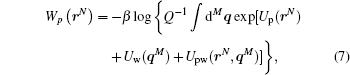
where Q is the configurational integral of the joint protein-solvent system, Up, Uw, and Upw are potentials of protein, that of water and their interaction, respectively. By keeping only averaged effects an approximation like the mean-field theory can be developed.
The interpretation of probabilities by taking their negative logarithms as potentials is convenient. Correlations among variables are converted to interactions in potentials. To include as many as possible important correlations is essential for estimates of probabilities. However, it should be emphasized that the correlations we can infer are dependent on the sample size. For a small sample size we cannot distinguish a sampling fluctuation from a true correlation.
As mentioned above, a protein is modeled as a mixture of multi-component molecular species. We usually use coarse-grained representations of polypeptide chains. We reduce the protein structure into units or centers of residues, or other types of simplified structural units, depending on how the specific models are constructed. Such centers are regarded as various molecular species, and their spatial distances are grouped into few bins.[6, 7]
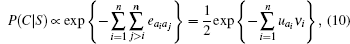
In the simplest model a residue is represented by just one center, and there are only two distance bins, i.e. ‘ contacted’ and ‘ non-contacted’ with respect to a cut-off distance or some other criteria.[8] The Miyazawa-Jernigan (MJ) contact potential for globular proteins is a widely used knowledge-based potential built on such a model.[9, 10] The MJ potential has only 210 energy values eab to characterize the tendency of a residue of identity a in contact with another residue of identity b in a native structure. There is an additional parameter of the cut-off distance for the contact definition. The probability for a conformation C of a chain with sequence S = a1a2… an to be native is estimated as

where χ i j is the characteristic function of contact, i.e. χ i j = 1 if residues i and j are in contact, and χ i j = 0 otherwise. In terms of distance ri j, cut-off rc, and the step function Θ , we have χ i j = Θ (rc – ri j).
In the MJ potential all correlations higher than two-body ones have been ignored. Furthermore, the additivity of the energy terms implies that each residue pair contributes P(C|S) independently. This independency assumption is one of the most important issues in the potential construction. A more general form of potential could be

where one-body term ha, σ may be interpreted as an external field exerting on a residue (or one of its representative centers) with feature or descriptor σ , the characteristic function χ a, σ (ai, σ i) = δ aaiδ σ σ i, and the meaning of τ is analogous to σ . An example of σ is the binary partition of residues as ‘ exposed’ and ‘ buried’ according to the accessible surface area or number of surrounding neighbors inside a cut-off sphere, and an example of τ could be the pair spatial distance, hydrogen-bonding status, or the secondary structure categories of the pair.
Generally, one-body terms contain the least number of parameters, and hence can be estimated most reliably. By an eigenvalue decomposition analysis of the 20× 20 symmetric matrix representing the MJ potential, it is found that contact energies eab are, in fact, dominant by the ‘ one-body’ desolvation terms.[11] This can also be verified by a parameter fitting.[12] Thus, it is advisable to first extract one-body terms and then include two-body terms as further corrections in constructing potentials.
After taking eab = ua + ub as a good approximation, the probability for structure C of sequence S to be native is estimated as
where ν i is the number of residues in contact with ai. A direct derivation of the one-body ua in the framework of the MJ potential model is given in Ref. [13].
(From the probabilistic viewpoint, an approximation of the joint probability P(C, S) under an independency assumption may be written as

which may be interpreted as a mean field approximation. To include correction from two-body correlation, we may write

where we have assumed that the combination (σ i, σ j) is consistent with τ i j. If the one-body independency assumption is valid, factors of the product inside the square bracket are of value 1, the one-body form (11) is then recovered. Here, exponent 1/ν i is added to remove multi-counting of pair effects, but need not be optimal. The pair corrections here will be converted to pair interaction in potentials. It should be mentioned that to avoid multiple counting of one and the same effect is rather tricky.
In real cases, independency assumptions are usually not valid. However, conditional independency can still be found as good approximations by designing features or descriptors carefully according to the nature of problems. For example, after a structure is referred to as a sequence {ν i} of coordinate numbers, usually we do not have the independency for the joint probability P(C, S), i.e., P(C, S) ≠ ∏ iP(ai, ν i), since the relation among ν i’ s is extremely intricate. However, P(S|C) = ∏ iP(ai|ν i), which well catches the main effects of hydration, could still be a good approximation.
How can we examine the validity of independency of a given model? Suppose that a good set of representative proteins is given, which are extracted from various types of structures, and any two samples from the set are not too similar either in sequence or in structure. With such a set we can easily estimate the probability of an amino acid, say alanine (A):

where N(x) denotes the total number of residues of amino acid type x in the set. The normalization constraint ∑ xP(x) = 1 makes only 19 of the 20 parameters being free. With a subset obtained by randomly choosing samples from the full set the estimated amino acid frequencies, which are now denoted by Q(x), will change little. A convenient measure of distance between two distributions P(x) and Q(x) is the Kullback-Leibler divergence defined by

which is known also as relative entropy, and is non-negative (and asymmetric between P and Q).[14] Under the assumption that both distributions P and Q are close, the leading term of D(P, Q) is a χ 2 variable.[15] (A χ 2 variable with k degrees of freedom is a sum of the squares of k independent standard normal random variables.) Considering the above binary partition of residues into ‘ exposed’ (e) and ‘ buried’ (b), we may estimate two amino acid distributions Pe(x) and Pb(x) conditional on the two categories (with descriptors σ ∈ {e, b}). The difference between Pe(x) and Pb(x) or D({Pe(x)}, {Pb(x)}) is large: hydrophobic residues have high values of Pb(x) while values of Pe(x) are high for polar ones, showing the hydration effect. This indicates the strong correlation between the hydrophobicity and environmental class of residues. There are many standard tests on statistical independency. The log-linear analysis is a useful for constructing potentials in this respect.[16, 17]
The standard statistical mechanics of a simple gas (of single component without any internal degree of freedom) in equilibrium starts with a pairwise additive potential

where u(ri − rj) ≡ ui j is the ‘ naked’ interaction between particle pair i and j. The Boltzmann distribution is P(rN) ∝ exp{− β U(rN)}. The potential w2(r1, r2) associated with the reduced pair distribution n2 in Eq. (6), as a potential of mean force, contains the effect of all other particles. Usually, w2 does not possess the additivity. Pair distribution n2 (and hence w2) can be directly extracted from a sample set, but it is usually rather complex to infer u2. A well-developed theory relating u2 to w2 is the Ornstein– Zernike equation together with an appropriate closure relation (which looks like the Dyson equation G = G0 + G0Σ G for Green’ s function).[18] This idea has been used to compute the effective potentials between amino acid residues.[19] A simple example to illustrate the difference between u2 and w2 is the multi-variate normal distribution where the latter corresponds to the variance, and the former to correlation parameters of the distribution. They are related as inverse of matrices.[20, 21]
A main goal of constructing potentials for proteins is to determine the native structure of a protein from its sequence. In order to understand how a protein folds to its native structure, we require that potentials should dynamically work, so that they can be used in a simulation like molecular dynamics to mimic the folding process. We are still in a position somewhat far from this intriguing destination. In most cases, potentials are used ‘ statically’ to discriminate between native and non-native conformations. For such a purpose, potentials are essentially the effective ‘ free energies’ of native structures with respect to certain reference conformations, or energy differences between native and reference structures. One direct way is to construct potentials separately for native and reference structures and then take their difference. However, there are alternatives based on optimization under some criteria, e.g., maximal energy gap between known native conformations and decoy ones. Such potentials depend not only on native structures, but also on decoy structures in given training sets. It should be emphasized that to create a set of reference conformations for a general purpose is by no means a simple task.
The advantage of knowledge-based energy functions is that they can model any behaviors seen in known protein structures, even if a good physical understanding of the behavior does not exist. However, a good physical understanding is always helpful in designing as simple as possible models of conditional independency to include important correlations. Recently, a simple and efficient statistical potential was reported, which has only a limited number of parameters but performs with an unprecedented reliability.[22] When constructing the potential, the one-body feature is also the above σ ∈ {e, b}. The energy term, say ue(a) for amino acid a being ‘ exposed’ , is estimated as

where the joint probability P(a, e) of amino acid a with feature e, and marginal probabilities P(a) and P(e) are inferred from the total number 

(Note that the independency P(a, e) = P(a)P(e) would imply ue(a) = 0.) The feature τ used for constructing pair energies is five classes of hydrogen-bonding statuses. Similarly, the pair energies are given by uτ (a, b) = − log [P(a, b|τ )/P(a, b)]. The disadvantage of knowledge-based potentials is that they are phenomenological and then hardly predict new behaviors absent from the training set.
Another problem related to the protein folding is the protein design.[23] Rational protein design approaches make protein-sequence predictions that will fold to specific structures. It is then also referred to as inverse folding: an unknown sequence is found to fold to a known conformation. The number of possible protein sequences is enormous, growing exponentially with the length of the protein chain, only a subset of them will fold reliably and quickly to a single native state. With a potential function given, a sequence ‘ mounted’ on the target structure has a value of energy. In an ideal case, such energy values will form a normal-like distribution. Candidate sequences are expected to fall in the lower tail of the distribution. The space spanned by random sequences is not physical. Thus, we do not have the Boltzmann distribution in a rigorous sense. The tail of extremely low energies of the candidate sequences usually has an exponential form, which is described by the theory of large deviations.[24] A parameter of the so-called rate function appears, playing a role of temperature in the Boltzmann distribution, but having nothing to do with a real temperature.[25]
The discovery of patterns or signals shared by several sequences that differ greatly is a basic task in biological sequence analysis, and still a challenge. For example, a class of gene regulation proteins contains the helix-turn-helix (HTH) motif for DNA binding as a signal with a width of about 18 residues. A simple model describing a signal or a portion of local multiple sequence alignment is the position-specific weight matrix (PSWM) model, in which a signal is characterized with position-specific probabilities. Thus, the HTH signal may be represented with a matrix M = (Pα i)20× 18, where entry Pα i indicates the probability for amino acid of type α to occur at position i of the motif. Generally, a signal is recognized with respect to a noise or background. The simplest model for the background is a position independent distribution {Qα }. According to the inverse Boltzmann principle, we introduce two sets of energies: {wi(α ) = − logPα i} and {b(α ) = − logQα }. We imagine that a residue may be painted either ‘ white’ or ‘ blue’ , and then it acquires an energy w or b. Assume that a sequence set sharing a signal is given, and the two sets of energies are known. For a ‘ coloring’ of a sequence from the set, we may compute its total energy. By finding the coloring whose total energy is minimal, the signal location on that sequence is determined. On the other hand, if the signal position of each sequence is known, i.e. all the sequences have been aligned according to the signal region, we may infer the two sets of energies. However, at the beginning we know neither the energies (Hamiltonian of the system) nor the signal positions on each sequence. We have to solve the problem self-consistently. A common way to break the loop is to make a random initialization. However, we make some guesses based on our previous knowledge.[26, 27] The signal discovery is then to minimize the total energy of all sequences in the set. The above discussion may be generalized to various cases. For example, sequences may share multiple signals, and a signal may be either present or absent or repeated in certain sequence. From the energetic viewpoint, pairwise sequence alignment may be thought of as a chain of one sequence in an external potential generated by the other sequence.
Relevant timescales for protein folding span over many orders of magnitude: from femtoseconds for bond-vibration, picoseconds for isomeration, nanoseconds for water dynamics and helix formation, to milliseconds for typical folders. This is one complexity of the protein folding. Thus, it is reasonable to build several models, each of which catches a certain nature of protein at a specific range of timescales. Associated with each model are certain levels of coarse-graining and corresponding potential functions. For example, to determine the packing of secondary structure elements of a protein (or its structural topology) is essential for structure prediction. So far, no potentials are particularly built and work for this purpose. There are fields for physics to display its prowess.
| 1 |
|
| 2 |
|
| 3 |
|
| 4 |
|
| 5 |
|
| 6 |
|
| 7 |
|
| 8 |
|
| 9 |
|
| 10 |
|
| 11 |
|
| 12 |
|
| 13 |
|
| 14 |
|
| 15 |
|
| 16 |
|
| 17 |
|
| 18 |
|
| 19 |
|
| 20 |
|
| 21 |
|
| 22 |
|
| 23 |
|
| 24 |
|
| 25 |
|
| 26 |
|
| 27 |
|