Structural modeling of proteins by integrating small-angle x-ray scattering data
[Zhang Yong-Hui, Peng Jun-Hui, Zhang Zhi-Yong† ]
]
]
|
|


†Corresponding author. E-mail: zzyzhang@ustc.edu.cn
*Project supported by the National Key Basic Research Program of China (Grant Nos. 2013CB910203 and 2011CB911104), the National Natural Science Foundation of China (Grant No. 31270760), the Strategic Priority Research Program of the Chinese Academy of Sciences (Grant No. XDB08030102), and the Specialized Research Fund for the Doctoral Program of Higher Education of China (Grant No. 20113402120013).
Elucidating the structure of large biomolecules such as multi-domain proteins or protein complexes is challenging due to their high flexibility in solution. Recently, an “integrative structural biology” approach has been proposed, which aims to determine the protein structure and characterize protein flexibility by combining complementary high- and low-resolution experimental data using computer simulations. Small-angle x-ray scattering (SAXS) is an efficient technique that can yield low-resolution structural information, including protein size and shape. Here, we review computational methods that integrate SAXS with other experimental datasets for structural modeling. Finally, we provide a case study of determination of the structure of a protein complex formed between the tandem SH3 domains in c-Cb1-associated protein and the proline-rich loop in human vinculin.
Large biomolecules such as proteins perform a variety of functions within living organisms, including catalysis of metabolic reactions, DNA replication, and molecular transport. To fully understand protein function, it is important to determine protein structure.[1] Currently, four major techniques are used for structural elucidation: X-ray crystallography, nuclear magnetic resonance (NMR), cryo-electron microscopy (cryo-EM), and SAXS. These techniques can help determine protein structure at either high or low resolution. SAXS is a promising technique that can rapidly provide global structural information, including protein size and shape.[2, 3] In addition, SAXS is useful in characterizing the flexibility of a protein in solution, because the scattering profile is the average of the multiple protein conformations present in the population. Due to its low-resolution nature, SAXS is usually used to complement high-resolution techniques. In such applications, termed “ integrative structural biology” , [4] computer simulations play an important role in combining SAXS and other experimental data. This review will introduce various computational methods for integrative modeling, which are aimed at determining the structures of proteins and investigating their flexibility in solution. To demonstrate the advantages of this hybrid strategy, at the end of the review we present our recent study, in which we determined the structural ensemble of a protein complex formed between the tandem SH3 domains of c-Cbl-associated protein and the proline-rich loop in human vinculin.
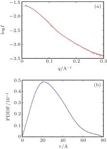
In a SAXS experiment, a protein sample is illuminated by x-rays, and the scattering intensities are recorded by a detector as a function of the scattering angle (typically 0.1° to 10° ). Because the sample solution is isotropic, the two-dimensional image obtained can be converted into a one-dimensional profile I(q) (Fig. 1(a)). The magnitude of the scattering vector q is 4π sin (θ )/λ , where 2θ is the scattering angle and λ is the x-ray wavelength. The radius of gyration (Rg) of the protein can be estimated directly from small q values using Guinier approximation, 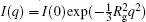
 | Fig. 1. Experimental SAXS data for the CAP-SH3ab:vin857 complex. (a) The SAXS scattering profile of the complex and (b) the corresponding PDDF curve. |
To integrate experimental SAXS data into structural modeling, one must be able to compute the theoretical SAXS profiles of the protein conformations generated by the simulation. Several programs are available that can calculate a SAXS profile from a protein structure, [9– 18] and they employ different methods for spherical averaging, as well as treatment of the excluded volume and the hydration layer.
Because proteins are randomly oriented in solution, spherical averaging is required in the calculation of the theoretical SAXS profile. For spherical averaging computation, CRYSOL[9] employs multipole expansion to accelerate calculation whereas fast-SAXS[13] and FoXS[15] use the Debye formula of pairwise inter-atomic distances. In CRYSOL, the atomic structure of the protein must be provided. To increase the computational efficiency, fast-SAXS defines a residue-level coarse-grained (CG) model of the protein, whereas FoXS accepts either an atomistic or a CG representation. Solute molecules are surrounded by a hydration layer and exclude a certain volume of bulk solvent, and both need to be taken into account. Programs like CRYSOL and FoXS treat the hydration layer implicitly, that is to say, the protein is assumed to be surrounded by a continuous envelope of adjustable density. The hydration layer can also be treated explicitly; for example, in Fast-SAXS, water molecules are introduced during the calculation. The excluded volume term is typically related to the shape of the molecule. CRYSOL calculates this portion of the scattering by assuming that the electron density of the excluded volume is equivalent to that of the bulk solvent. Because the total volume varies depending on a set of atomic radii values, accurate computation of the excluded volume is difficult. Therefore, CRYSOL and FoXS allow adjustment of the excluded volume of the protein for optimal fitting of the experimental SAXS profile.
Usually, the theoretical SAXS profile is fitted to the experimental profile by minimizing

where Iexp(q) and I(q) are the experimental and theoretical scattering profiles, respectively, σ (q) is the experimental error, M is the number of data points in the profile, and c is the scaling factor.
To integrate low-resolution SAXS data into structural modeling of proteins, two strategies are generally applied: refining while sampling and screening after sampling.[19]
If a high-resolution structure is not available for a protein (or protein complex) that has a dominant conformation in solution, an atomic model of the protein can be built by refining the structure against the experimental SAXS data. These refining-while-sampling approaches take SAXS and other chemical information into account simultaneously, to determine the solution structures of multi-domain proteins or protein complexes.
BUNCH and SASREF[20] are two programs in the ATSAS package[21] that are used for modeling the structure of multi-domain proteins and multi-subunit complexes, respectively. Individual domains (subunits) are treated as rigid bodies. Starting from an initial arrangement of domains (subunits), a simulated annealing (SA) protocol is employed to determine the positions and orientations of the domains (subunits) without steric clashes, while minimizing the discrepancy between the calculated and the experimental scattering profiles. Other data, such as known interfaces between domains (subunits), can be considered by restraining the inter-residue distances accordingly. Rigid body modeling and the SA protocol are also used in xplor-NIH[22] for refining protein structures to best reproduce the SAXS and NMR data. SAXS data can also be integrated into docking methods that use rigid body global searching and local interface complementary minimization. By optimizing the relative weighting of experimental and theoretical potentials, pyDockSAXS combines SAXS data and protein– protein docking methods for complex building.[23] It uses FTDock for sampling the orientations of subunits, [24] pyDock for energy-based scoring, [25] and CRYSOL for SAXS profile calculation. In FoXSDock, [26] complex models are generated by rigid global docking using PatchDock.[27] The models are filtered and clustered based on the experimental SAXS data and the theoretical profiles computed by FoXS. The interface is refined by flexible docking using the FireDock package.[28]
Rigid body modeling is widely used for its speed and efficiency, but protein domains (subunits) can be flexible and undergo conformational changes. In these cases, flexible fitting methods are used to study the conformational transitions of proteins in solution, combined with SAXS data. In a coarse-grained elastic network model for flexible fitting developed by Zheng and Tekpinar, the known high-resolution structure is flexibly fitted to the low-resolution SAXS data using computer simulations.[29] The fitting procedure is based on a coarse-grained protein representation and a modified elastic network model, allowing large-scale conformational changes while preserving pseudo-bonds and secondary structures. Normal mode flexible fitting iteratively uses a linear combination of low-frequency normal modes from the elastic network model of the protein, in order to optimize the structure toward the target PDDF obtained from the SAXS profile.[30] An optimization algorithm called the trusted region method is employed.
X-ray scattering-guided molecular dynamics (XS-guided MD) simulation is a newly develop method[31] that combines the information encoded in time-resolved SAXS curves with chemical data from molecular force fields. Using the Debye scattering equation, XS-guided MD adds a restraint energy term to the conventional MD potential energy function, in order to guide the simulation toward states that match the experimental data. The simulation is biased toward the experimentally observed conformational space, and alternative conformations with similar free energies can be distinguished.
A protein that is highly flexible in solution is better described by a structural ensemble than by a single dominant conformation.[32] In this case, some screening-after-sampling approaches have been proposed for determining the ensemble using SAXS data. In these approaches, sampling and comparison with the experimental data are performed sequentially. First, a pool of structures is generated, which contains a large number of candidate conformations to cover the configurational space of the protein. Several methods are available for pool generation, such as rigid body modeling, [8] MD simulations, [33] enhanced sampling methods, [34] and CG simulations.[35, 36] Then algorithms are applied to select a representative ensemble with the best fit (the minimal χ value) to the experiment SAXS profile.
The EOM is one such approach.[8] The program Pre_ bunch[20] is used to generate a pool of structures for flexible multi-domain proteins using rigid-body modeling. Typically, a large number of structures (105) are generated, and then the scattering profile of each structure is calculated by CRYSOL. A genetic algorithm is employed for screening of the pool. An ensemble containing a number of different conformations, with an average scattering profile that best fits the experiment data, is selected to represent the flexible protein in solution. Recently, our group implemented an enhanced sampling technique, termed amplified collective motions (ACM), to generate the pool of protein structures for SAXS fitting.[34]
In BILBOMD, [33] a rigid-body MD simulation is used to explore the conformational space of a flexible protein, during which high temperature is introduced to linkers between domains to prevent trapping in local minima and non-bonded interactions are simplified to reduce computational cost. Minimal ensemble search (MES) is performed for ensemble selection, using a genetic algorithm. To avoid over-fitting, two to five representative conformations are selected from the pool of structures to reproduce the experimental SAXS data.
Basis-set supported SAXS (BSS-SAXS) is another screening-after-sampling approach.[35] A pool of structures is generated through extensive CG simulations, and the theoretical SAXS profile of each conformation is computed using fast-SAXS. Then the conformations are clustered by inter-domain pair-wise residue distances and SAXS profile similarity using the K-means algorithm, [36] to form a small number of assembly states called a basis-set. Finally, the fractional population of these states is determined via a Bayesian-based Monte Carlo analysis that seeks to optimize the theoretical scattering profile against the experimental SAXS data. Similarly, the ensemble refinement of SAXS (EROS) method utilizes a CG model of protein binding to generate a large pool of protein conformations via replica exchange Monte Carlo simulations.[37] Then the simulated structures are clustered using the QT-clustering method, using distance root-mean-square as a metric.[38] The arithmetic mean of the SAXS intensities of each cluster (conformational state) is calculated, and the maximum-entropy method is implemented to refine the relative weight of these states, to improve agreement with the experimental SAXS data.
Because it is challenging to elucidate the structure of flexible multi-domain proteins or protein complexes using a unitary technique, hybrid approaches have been developed that integrate relatively high-resolution data from x-ray crystallography, NMR, or cryo-EM with low-resolution data from SAXS and other experiments. These methods benefit from employing various experimental datasets, including the atomic structures of domains (subunits) solved by x-ray crystallography or NMR, global structural information from SAXS, interface information from chemical shift perturbations[39] or mutational analysis, orientation of domains (subunits) from residual dipolar couplings, [40] and others. As an example, the integrative modeling platform (IMP) treats the building of protein structural models as a computational optimization problem.[41] A scoring function is created to evaluate candidate models at the atomic or CG level. Structural information from different sources including SAXS profiles is encoded into the scoring function (based on the FoXS method). The generated models are tested and refined using additional structural data, until a convergent ensemble of models is reached.
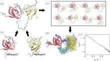
c-Cbl-associated protein (CAP) is an important cytoskeletal adaptor that functions in the regulation of adhesion turnover.[42] It consists of a SoHo domain and three tandem SH3 domains. Human vinculin is comprised of a head domain and a tail domain connected by a proline-rich region (prr).[43] It has been reported that binding of the first two SH3 domains of CAP (called CAP-SH3ab) to the prr of vinculin is responsible for localization of CAP for cell-extracellular matrix adhesion.[44] The crystal structure of the isolated SH3a domain in complex with residues 870– 879 of vinculin (called prr2) has been solved to a resolution of 1.41 Å (pdb code 4LNP), along with that of the isolated SH3b domain in complex with residues 858– 867 of vinculin (called prr1) with a resolution of 1.00 Å (pdb code: 4LN2) (Fig. 2(a)). However, because the prr domain of vinculin is highly flexible, it is difficult to obtain the combined crystal structure of the tandem SH3ab complexed with the C-terminal prr of vinculin (residues 857– 879, denoted as vin857). We determined a structural model of this complex by combining high-resolution structures of SH3a:prr2 and SH3b:prr1 with SAXS data for the complex via computational simulation using a structure-based model (SBM). A flow chart of the model building process is shown in Fig. 2.
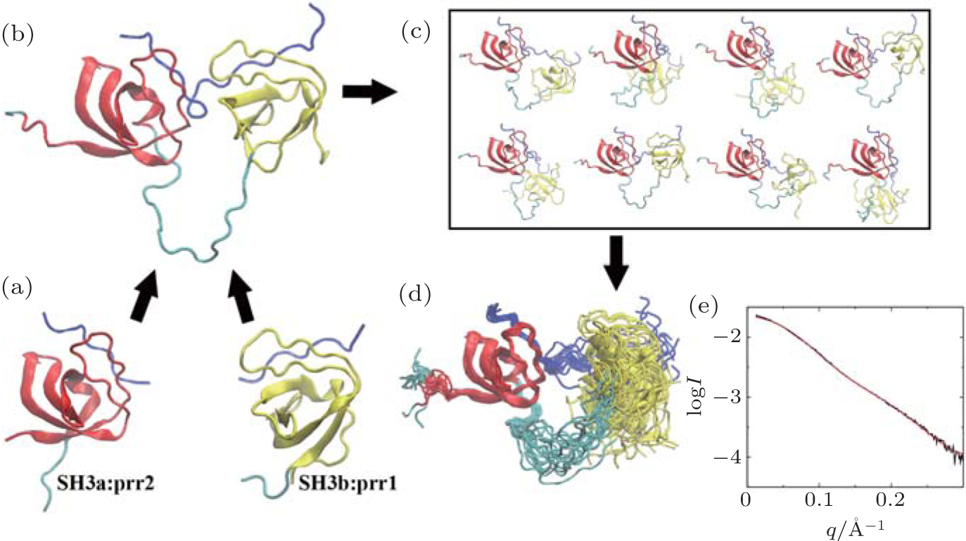 | Fig. 2. A flow diagram of the process of building the model of the CAP-SH3ab:vin857 complex. (a) Crystal structures of SH3a:prr2 and SH3b:prr1. The SH3a and SH3b domains are shown in red and yellow, respectively, whereas prr1, prr2, and vin857 are shown in blue. (b) The initial structural model of the CAP-SH3ab:vin857 complex. (c) Pool of conformations of the complex generated by MD simulations, using an all-heavy-atom SBM. (d) The EOM ensemble selected from the conformation pool. (e) The SAXS curve calculated (red solid line) for the EOM ensemble with χ = 0.26, compared to the experimental SAXS profile (black solid line). All structures were created using VMD.[50] |
The SAXS data for the CAP-SH3ab:vin857 complex were collected at beamline 12ID-B of the Advanced Photon Sources (APS) at Argonne National Laboratory (Chicago, IL, USA) using a wavelength of 1.033 Å . The data were analyzed using the ATSAS package.[21] The radius of gyration (Rg) of the protein, calculated from the PDDF (Fig. 1(b)), is approximately 22.5 Å .
An initial structure for the vin857 peptide was first built by homology modeling, in which the structures of prr1 and prr2 were taken from the crystal structures of SH3b:prr1 and SH3a:prr2, respectively (Fig. 2(a)). It was then straightforward to dock the SH3a and SH3b domains on the vin857 peptide, and an initial model of the CAP-SH3ab:vin857 complex was obtained (Fig. 2(b)).
The configurational space of the complex was explored via CG MD simulations using an all-heavy-atom SBM (Fig. 2(c)).[45] By loading the initial structure of the complex on the SMOG web server, [46] topology and coordinate files were generated for the MD simulations using the GROMACS-4.5.5 package.[47] The native contacts were defined using a shadow algorithm.[48] To facilitate sampling of possible conformations, all stabilizing contacts were removed from the topology file, except those present in the crystal structures SH3a:prr2 and SH3b:prr1. Two independent MD simulations with different initial atomic velocities were performed. Each simulation was coupled to a temperature bath of 50.0 in reduced units via Langevin dynamics. A time-step of 0.002 time units was used and the total simulation time was 105 time units, which corresponds to approximately 500 microseconds.[49]
The EOM was used to screen for conformations in the MD trajectories that fit the SAXS data for the complex. In the ensemble chosen from the first simulation (Fig. 2(d)), the Rg values were between 21.4 Å and 23.8 Å , with an average of 22.1 Å . The theoretical SAXS profile was concordant with the experimental curve, with χ = 0.26 (Fig. 2(e)). The ensemble from the second simulation (data not shown) contained conformations with Rg ranging from 21.1 Å to 24.2 Å (the average was also 22.1 Å ), with χ = 0.26 when fit with the experimental data. The two independent simulations can yield similar results via EOM analysis, which indicate the ensemble shown in Fig. 2(d) is reliable. The theoretical scattering profile of each conformation in the MD trajectories was computed using CRYSOL. Fitting with the experimental SAXS data, all χ values of theoretical profiles were > 1.0. This result suggests that the CAP-SH3ab:vin 857 complex is flexible in solution, and that it would therefore be better represented as an ensemble instead of as a single dominant conformation.
Structural modeling methods that integrate SAXS data have been established, and this strategy shows promise for constructing structural models of proteins. One important issue for these screening-after-sampling approaches is to generate a pool of structures that adequately covers the configurational space of the protein. Therefore, the algorithms need to be improved to accelerate sampling efficiency. Although it is efficient to determine the structures of large multi-domain proteins or protein complexes using SAXS-integrated structural modeling methods, it should be noted that the resolution of SAXS data is inherently low, which may lead to ambiguous results. To tackle this over-fit problem, efforts should be made to improve the algorithms used in the screening step. Use of experimental data from other techniques, such as mass spectrometry and cross-link experiments, in addition to SAXS data may be helpful in distinguishing these ambiguous structural models. Future research should investigate combining these methods with other low-resolution datasets for validation.
| 1 |
|
| 2 |
|
| 3 |
|
| 4 |
|
| 5 |
|
| 6 |
|
| 7 |
|
| 8 |
|
| 9 |
|
| 10 |
|
| 11 |
|
| 12 |
|
| 13 |
|
| 14 |
|
| 15 |
|
| 16 |
|
| 17 |
|
| 18 |
|
| 19 |
|
| 20 |
|
| 21 |
|
| 22 |
|
| 23 |
|
| 24 |
|
| 25 |
|
| 26 |
|
| 27 |
|
| 28 |
|
| 29 |
|
| 30 |
|
| 31 |
|
| 32 |
|
| 33 |
|
| 34 |
|
| 35 |
|
| 36 |
|
| 37 |
|
| 38 |
|
| 39 |
|
| 40 |
|
| 41 |
|
| 42 |
|
| 43 |
|
| 44 |
|
| 45 |
|
| 46 |
|
| 47 |
|
| 48 |
|
| 49 |
|
| 50 |
|