Consider the time-dependent Hamiltonian

where

where h.o.t. denotes the high order terms of z⁴, α (t) and β (t) are continuous 2π -periodic functions, which characterise the strength of the nonlinearities. The lattice dynamics corresponding to Hamiltonian (1) is governed by the following system of coupled equations

where q_j denotes the displacement of the j-th oscillator with respect to its rest point position.

When H is independent of time, equation  (2) is called a Fermi– Pasta– Ulam (FPU) system which was initially introduced to answer various sophisticated questions related to irreversible statistical mechanics and to test the simplest and most widely believed assertions of equilibrium statistical mechanics such as equipartition of energy, ergodicity by Fermi, Pasta, and Ulam in 1955.^[1] The chain is called an α -chain if β ≡ 0, α ≠ 0 and a β -chain if α ≡ 0, β ≠ 0.^{[2, 3]} Starting from the first numerical results of FPU, both theoretical and numerical findings are discussed in close connection with the problems of ergodicity, ^{[4, 5]} integrability, ^{[6, 7]} chaos and stability of motion.^{[8– 13]}

The FPU model with the time-dependent nonlinear term is used to explore the relation between the thermodynamic entropy change due to irreversible processes and the change of information loss as a chaotic dynamical system (see Ref.  [14] for instance). Although the time-dependent FPU Hamiltonian  (1) can be considered as a perturbation of the harmonic oscillator by rescaling a small parameter, q_j ↔ ϵ q_j, the dynamics of inharmonic lattices display a rich variety of features: periodic motions, ^{[15– 17]} quasi-periodic invariant tori, ^[18] discrete solitons and breather.^{[19– 21]} Motivated by the recent paper, ^[17] where the authors prove the existence and multiplicity of periodic solutions of Eq.  (2) under certain appropriate conditions with non-identical action potential V, we perform the calculation of periodic orbits and study their stability by the averaging theory for the three particles time-dependent FPU chains. Compared with Ref.  [17], where the potentials have a linear growth at infinity, the classical model  (2) does not meet the conditions in this case. The objective of this paper is to provide a system of nonlinear equations whose simple zeros provide periodic solutions of Eq.  (2).

The rest of this paper is organized as follows. We shall present the basic results from averaging theory in Section  2 and introduce the procedure of reducing to standard form in Section  3. Finally, in Section  4 we shall apply these theories to three particles time-dependent FPU chains where the period of α , β taken by is resonant with the basic frequency. For autonomous three particles FPU chains, the α -chain is completely integrable and the Hamiltonian of the β -chain can be identified with the Hé non– Heiles Hamiltonian. To some extent, the existence of all these periodic solutions is attributed to the existence of resonance terms for α and β . We find nine periodic solutions with six of them being unstable when we take the “ test” functions for any α ₀ ∈ ℝ and β (t) = 1; we obtain seventeen periodic solutions with fifteen of them being unstable while specifying and .

The method of averaging is a transformation procedure leading to a systematic perturbation expansion complete with error bounds on the difference between exact and approximate solutions, ^[22] and it is an important tool in the rigorous study of differential equations with a small parameter for proving properties of the exact problem based on properties of the approximate problem. A good example of applying the method of averaging to a beam dynamics problem is given by Ellison and Shih.^[23]

Consider the following system of the standard form of averaging

where f : ℝ × Ω × [0, 1] → ℝ ⁿ is C^r(r ≥ 1), bounded on bounded sets and T-periodic in t, and Ω is a bounded and open subset of ℝ ⁿ. The associated autonomous averaged system is defined as

Now we state the averaging theorem, and the proof can be found in Refs.  [24] and [25].

Theorem 1 (averaging theorem) There exists a C^r change of coordinates x = x̄ + ϵ w(t, x̄ , ϵ ) under which equation  (3) becomes

where f : ℝ × Ω × [0, 1] → ℝ ⁿ is T-periodic in t. Moreover:

(i) If x(t) and x̄ (t) are solutions of Eqs.  (3) and (4) with the initial values x(t) = x₀ and x̄ (t) = x̄ ₀, respectively, and then on a time scale t ∼ 1/ϵ .

(ii) If a₀ is a non-degenerate rest point of Eq.  (4), so that f̄ (ā ₀) = 0 and Df̄ (ā ₀) is nonsingular. Then there exists ϵ ₀ > 0 such that, for all 0 < ϵ ≤ ϵ ₀, equation  (3) possesses a unique T-periodic orbit x(t; a_ϵ , ϵ ) such that

(iii) If the rest point a₀ of Eq.  (4) is hyperbolic, then the T-periodic orbit x(t; a_ϵ , ϵ ) of Eq.  (3) is hyperbolic, and its unstable dimension is one greater than that of the rest point.

(iv) If x^s(t) ∈ W^s(x(t; a_ϵ , ϵ )) is a solution of Eq.  (3) lying in the stable manifold of the hyperbolic periodic orbit x(t; a_ϵ , ϵ ), x̄ ^s(t) ∈ W^s(a₀) is a solution of Eq.  (4) lying in the stable manifold of the hyperbolic fixed point a₀ and then for t ∈ [0, + ∞ ). Similar results apply to solutions lying in the unstable manifolds on the time interval t ∈ (− ∞ , 0].

We remark that in the change of coordinates, w(t, x̄ , ϵ ) is given by

Consider the system

where q, p ∈ ℝ ⁿ, A is a real n × n symmetric matrix and positive semi-definite, ϵ is a sufficiently small real parameter and h : ℝ × ℝ ⁿ × ℝ ⁿ × [0, ϵ ₀] → ℝ ⁿ is a smooth T-periodic function. We are concerned in this section with the procedure of reducing Eq.  (6) to standard form.

Firstly, since A is symmetric and positive semi-definite, it is always orthogonally diagonalizable and has only real and non-negative eigenvalues λ ₁, λ ₂, … , λ _n. Therefore, there exists an orthogonal matrix B such that BAB^T = Λ and B^TB = I, where Λ = diag(λ ₁, λ ₂, … , λ _n), I is the identity matrix and B^T denotes the transpose of matrix B. Now we take an orthogonal transformation by

and let i = 1, 2, … , then system  (6) becomes

where h̃ _i denotes the i-th row of the vector Bh.

Consequently, in case there exists i such that ω _i = 0 and h̃ _i(t, B^Tq̄ , B^Tp̄ , ϵ ) ≡ 0, we can solve q̄ _i(t) directly. For ω _i > 0, i ∈ {1, 2, … , n}, to obtain a system of a differential equation in the standard form for averaging, instead of amplitude-phase variables in the usual way we introduce the symplectic transformation by

which transforms system  (7) into

We denote the index sets by 𝓙 = {i : 1 ≤ i ≤ n, ω _i = 0}, respectively. We rescale for i ∈ 𝓙 , ū _i = q_i, for ū _j = ϵ ^{− 1/2}u_j, . Then we have the system in the standard form

Usually, system  (10) is a quasi-periodic system while the frequencies ω _i are rational independent. The form of averaging corresponds to taking quasi-periodic averaging. For seeking periodic solutions, we assume that all positive eigenvalues λ _i are identical so that ω _i ≡ ω , or all positive eigenvalues such that .

In this section, we take

where α , β are T-periodic functions with We may visualize the time-dependent FPU system (n = 3) as a perturbed linear system with, putting ϵ = 0, frequency It is apparent from the choice of the period T that the adjustable external frequency is resonant with the basic frequency. Then the time-dependent Hamiltonian is defined by

which corresponds to the Hamilton system

where the real 3 × 3 symmetric matrix A is given by

Obviously, A is positive semi-definite.

Now we take an orthogonal transformation by

then system (11) transforms into

In view of system  (13), since equations of q̄ ₃, p̄ ₃ are integrable, we drop these equations in the subsequent discussion. System  (13) has the periodic solution if and only if we take q̄ ₃ = p̄ ₃ = 0.

We introduce a symplectic transformation by

which transforms system  (13) into the standard form of averaging

where

4.1. Case I: β (t) = 1, ∀ α ₀ ∈ ℝ

Substituting β (t) = 1 into system  (15) and taking an average on a period T, we obtain the averaged equation

In order to find the rest points of system  (16), we have to solve the algebraic equations while letting the right-hand of system  (16) equal zero. It seems that the algebraic equations are very complicated, but it is easy to solve. We have found nine non-degenerate rest points listed in Table  1. From Table  1, we know that the real part of eigenvalues of Jacobi matrix corresponding to the first three rest points are zero, while the others are nonzero which implies these rest points are unstable. Applying the averaging theorem (see Theorem  1), we conclude our result in the following.

Table 1.

Table 1.

Table 1. Nine non-degenerate rest points of system  (16).

Table 1. Nine non-degenerate rest points of system  (16).

Theorem 2 For any real number α ₀, let β (t) = 1, and i = 1, 2, … , 9, be given in Table  1, then there exists ϵ ₀ > 0 such that, for all 0 < ϵ ≤ ϵ ₀, equation  (11) has at least nine nontrivial -periodic solutions satisfying that for i = 1, 2, … , 9,

Moreover, six of them (i = 4, … , 9) are unstable.

Proof Proceeding as discussed above, in view of Table  1, we have found nine non-degenerate rest points i = 1, 2, … , 9, of system  (16). Applying Theorem  1, there exists a constant ϵ ₀ > 0 such that, for all 0 < ϵ ≤ ϵ ₀, equation  (15) has at least nine nontrivial -periodic solutions satisfying that

Furthermore, for each i ∈ {4, … , 9}, the Jacobi matrix corresponding to rest point P_i has an eigenvalue with positive real part, which yields that periodic solutions (i = 4, … , 9) are unstable. System  (13) has the periodic solution if and only if we take q̄ ₃ = p̄ ₃ = 0. Now together with symplectic transformations (12) and (14) and returning to the original equation (11), we complete the proof of Theorem  2.        ◻

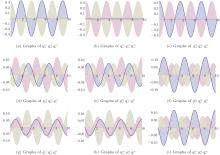
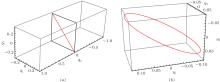
From Theorem  2, we know that the existence of periodic solutions of Hamilton system  (11) are unrelated to the choice of coefficient α ₀. In fact, for autonomous three-dimensional FPU chains, the α -chain, which does not contain a resonant term, is completely integrable. We plot the curves of periodic solutions in Fig.  1, and in Fig.  2 we plot the parametric curves generated by periodic solutions of system  (11) in the configuration space (q₁, q₂, q₃). From Fig.  2, we can see that the periodic solutions have two kinds of different properties: one kind of periodic solutions run linear motion (see Fig.  2(a)) while the other kind of periodic solutions move on a closed curve (see Fig.  2(b)) in the configuration space (q₁, q₂, q₃).

Fig.  1.

	Figure Option ViewDownloadNew Window
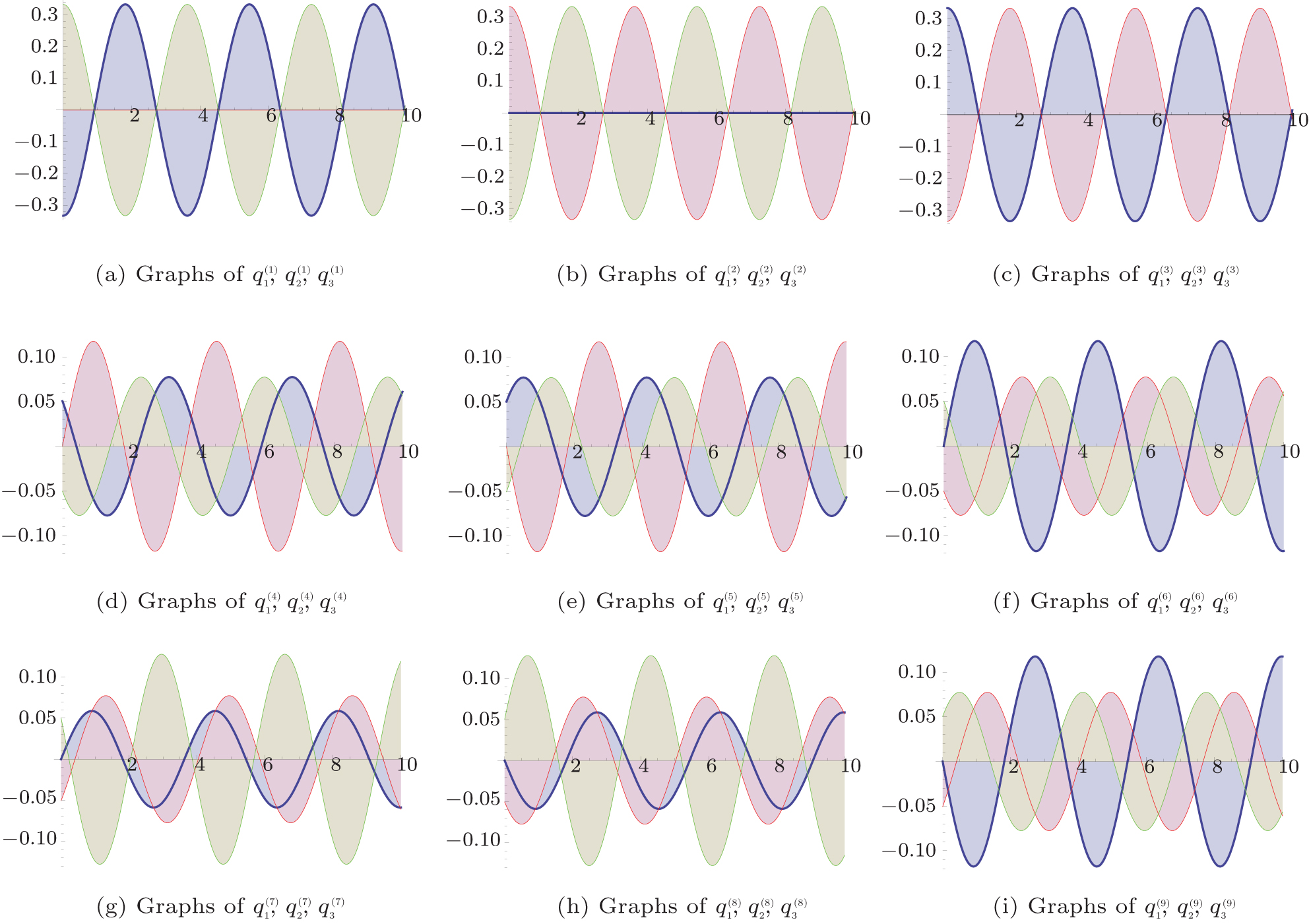	Fig.  1. The profiles of -periodic solutions of system  (11) with and i = 1, 2, … , 9.

Fig.  2.

	Figure Option ViewDownloadNew Window
	Fig.  2. The profiles of parametric curves generated by periodic solutions of system  (11).

In Fig.  1, all of the expressions for variables and are given as follows: (red), (green), (blue), i = 1, 2, … , 9.

4.2. Case II: ,

In this subsection, in order to investigate the variety of the number of periodic solutions, we add a resonant term for the coefficient β . Substituting , into system  (15), we obtain the averaged equation

Similar to the previous subsection, we obtain seventeen non-degenerate rest points for system  (17) listed in Table  2 and fifteen of them are unstable. By using an averaging theorem we conclude the result below without proof.

Table 2.

Table 2.

Table 2. Seventeen non-degenerate rest points of system (17).

Table 2. Seventeen non-degenerate rest points of system (17).

Theorem 3 Assume that , . Let , i = 1, 2, … , 17, be given in Table  2, then there exists ϵ ₀ > 0 such that, for all 0 < ϵ ≤ ϵ ₀, equation  (11) has at least 17 nontrivial -periodic solutions satisfying that, for  each i ∈ {1, … , 17},

Moreover, fifteen of them i ∈ {1, … , 17}\ {10, 13} are unstable.

We have used the averaging theory, one of the important tools in the area of dynamical systems, for studying analytically the existence of periodic orbits and their stability adapted to three particles time-dependent FPU chains. To some extent, the existence of all these periodic solutions is attributed to the existence of resonance terms for α and β . We have found nine periodic solutions with six of them being unstable when we take the “ test” functions , for any α ₀ ∈ ℝ and β (t) = 1, and obtained seventeen periodic solutions with fifteen of them being unstable when specifying and . The main results on the periodic orbits for three-dimensional time-dependent FPU chains are summarized in Theorem  2 and Theorem  3.

When considering the FPU model with a larger number of particles, we know that the linear spectrums, the frequencies of the normal models, are dense in the closed interval [0, 2]. There will occur multiple rationally independent frequencies, which leads to a quasi-periodic system. For instance, for FPU chains composed of four particles, the transformed systems have the linear spectrums 2 and . Therefore, the application of the averaging method for larger FPU systems becomes much more difficult, even for a theoretical point of view. This problem may be a good topic for further study, and we also expect some related results both on the theoretical and numerical aspects.