Exponential flux-controlled memristor model and its floating emulator*
[Liu Wei, Wang Fa-Qiang , Ma Xi-Kui]
, Ma Xi-Kui]
|
|


†Corresponding author. E-mail: eecjob@126.com
*Project supported by the National Natural Science Foundation of China (Grant Nos. 51377124 and 51221005), the Foundation for the Author of National Excellent Doctoral Dissertation of China (Grant No. 201337), the Program for New Century Excellent Talents in University of China (Grant No. NCET-13-0457), and the Natural Science Basic Research Plan in Shaanxi Province of China (Grant No. 2012JQ7026).
As commercial memristors are still unavailable in the market, mathematic models and emulators which can imitate the features of the memristor are meaningful for further research. In this paper, based on the analyses of characteristics of the q– φ curve, an exponential flux-controlled model, which has the quality that its memductance (memristance) will keep monotonically increasing or decreasing unless the voltage’s polarity reverses (if not approach the boundaries), is constructed. A new approach to designing the floating emulator of the memristor is also proposed. This floating structure can flexibly meet various demands for the current through the memristor (especially the demand for a larger current). The simulations and experiments are presented to confirm the effectiveness of this model and its floating emulator.
In 1971, based on the symmetry and the completeness of the circuit theory, Chua proposed that there should be a basic two-terminal circuit element characterized by a nonlinear relationship between the charge 
In spite of so many special features of the new basic element, there is no widespread attention until it was fabricated in HP labs in 2008.[4] After this remarkable work, more and more researchers make their effort to investigate the memristor, and a great number of valuable results have been obtianed in neural networks, [5– 8] computer memory, [9– 12] analog circuits, [13– 21] stochastic impulsive systems, [22] and so on.
As indicated in Ref. [23], an appropriate model of the memristor is necessary for the convenience of theoretical analysis. The memristor is divided into two categories: the charge-controlled memristor and the flux-controlled memristor.[1] For the former, the HP research team proposed a charge-controlled memristor model and its experimental verifying was also carried out.[4] Based on the HP Ti02 memristor, Joglekar and Wolf proposed a special window function which can ensure zero drift at the boundaries.[13] For the latter, Itoh and Chua presented a ‘ monotone-increasing’ and ‘ piecewise-linear’ q– φ function (PWL) in Ref. [24], and a cubic continuous nonlinear flux-controlled model was proposed in Ref. [25]. Additionally, it is known that commercial memristors are still unavailable in the market due to the cost and technical difficulties in fabricating nanodevices. Hence, a replacement which can imitate the features of the memristor is needed for further research. Several SPICE macromodels, which are very useful for simulating the memristor, were presented in Refs. [26]– [28]. Many excellent works on the hardware emulator which acts like a real memristor and lays a good foundation for experiments have also been reported.[29– 33] All of these are practically useful works and have made a great contribution to the research on the memristor.
However, there are still some deficiencies. For example, neither of the flux-controlled models in Refs. [24] and [25] are completely in line with the variation law that the memristance (memductance) should always keep increasing or decreasing (if not approach the boundaries) until the voltage’ s polarity reverses.[4] This imperfection may cause some inconvenience when the initial phase of the input voltage is changed. Besides, the input (output) currents of the previous emulators are too small (usually less than 10 mA), so they have limitations in those situations which demand a larger current. According to the definition of the memristor in Ref. [2], many devices are also considered as memristors because they possess the particular features of the memristor, such as gas discharge arcs, mercury lamps, etc.[2, 34– 36] Therefore, a flux-controlled model which has the quality that its memductance (memristance) will keep increasing or decreasing unless the voltage’ s polarity reverses (if not approach the boundaries) and a design of the memristor emulator which can meet various demands for the current through the memristor (especially the demand for a larger current) are of great significance to the research on the memristor. In this paper, a new flux-controlled model based on an exponential function is proposed and its corresponding floating emulator (allows a larger current) is also presented.
The remainder of this paper is organized as follows. The new exponential flux-controlled q– φ function is proposed and discussed in detail in Section 2. In Section 3, the design principle of the floating memristor circuit emulator is described, and some experimental results are presented. The conclusion is given in Section 4.
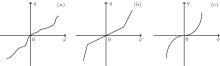
The characteristics of the memristor are determined by the relationship between the charge and the flux, which means that the q– φ curve should be identified at first.[1] From Refs. [1]– [4], the passive memristor is an energy dissipation element, and it cannot discharge or store energy. Thus, its q– φ curve must go through the origin. What is more, because the relationship between q and φ must be nonlinear (a linear relationship will make it a linear resistor) and actual elements always have boundaries, both M(q) and W(φ ) are positive and non-constant. As described above, the q– φ curve must be zero-crossing, monotonically increasing and nonlinear, as shown in Fig. 1(a).
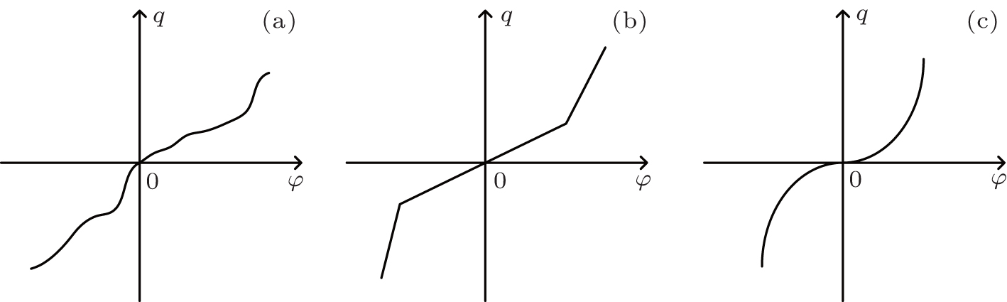 | Fig. 1. Schematic diagrams of the q– φ curve of the memristor. (a) Possible q– φ curve of the memristor. (b) The q– φ curve of the PWL model. (c) The q– φ curve of the cubic model. |
Up to now, the published papers on the flux-controlled memristor are mainly based on two models: the PWL model[24] and the cubic nonlinearity.[25] In other words, these two models have made a great contribution to the research on the memristor. As indicated in Ref. [4], if the memristance does not approach the boundaries, it will keep increasing or decreasing unless the voltage’ s polarity reverses. However, the variation laws of the memristances in the two models are not immutable with different excitation voltages. For example, the q– φ function of the cubic flux-controlled model is given by
 |
Then, the memductance W(φ ) can be obtained as
 |
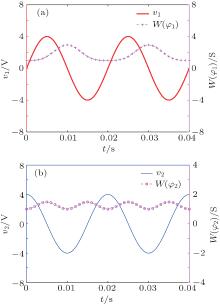
Let α = 1, β = 1000, and φ (t)| t= t0 = 0. As shown in Fig. 2, by applying the voltage v1 (v1 = Vm sin(2π ft)) to the memristor, the memductance will be monotonically increasing (decreasing) when the instantaneous value of v1 is positive (negative). However, the W(φ )– t curve will not be monotonic whether the terminal voltage is in the positive interval or the negative interval when the voltage equals v2 (v2 = Vm sin(2π ft + π /2)). In other words, the variation laws of the flux-controlled models’ memductances in Refs. [24] and [25] will not always be the same with different excitation voltages, so they have some limitations in applications. For instance, even though the polarity of the terminal voltage has been known, it cannot be easily determined whether the memductances are increasing or not.
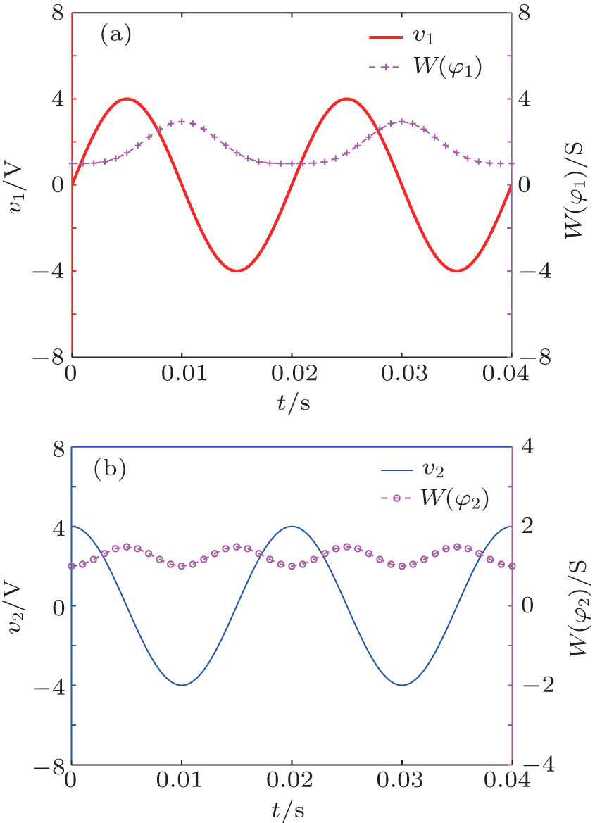 | Fig. 2. Time domain waveforms of the cubic model’ s memductance under different excitation voltages: (a) excitation voltage v1, (b) excitation voltage v2. Here Vm = 4 V and f = 50 Hz. |
The reason for this deficiency can be observed from their q– φ curves. The memductance W(φ ) (W(φ ) = dq(φ )/dφ ) is equal to the slope of the q– φ curve. As shown in Figs. 1(b) and 1(c), the slopes of the q– φ curves decrease (increase) gradually as φ increases when φ is less (greater) than 0. Besides, φ is the integral of the voltage 
To fix the above drawback of the former two models, we propose a novel model of the flux-controlled memristor, which is given by
 |
where a > 1, and kb > 0. Then, the memductance function of this memristor can be given by
 |
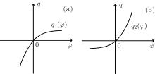
When b < 0, the model of Eq. (3) is a decremental flux-controlled memristor, that is, its memductance is monotonically decreasing (increasing) when the supply voltage is positive (negative), and its q– φ curve is shown in Fig. 3(a). On the contrary, when b > 0, equation (3) presents an incremental flux-controlled memristor and the corresponding q– φ curve is shown in Fig. 3(b). In other words, the proposed exponential model has a stable variation law of the memductance (memristance) under various excitation voltages.
 | Fig. 3. The q– φ curves of the proposed flux-controlled model: (a) decremental memristor, (b) incremental memristor. |
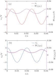
Here, the decremental memristor as an example is discussed in detail. The incremental memristor can be analyzed in the same way. Set the parameters as follows: a = e, b = 50ln(0.5), and k = − 1/(2500ln 2). Then, from Fig. 4, one can see that the memductance is monotonically decreasing (increasing) when the supply voltage is positive (negative) whether the voltage v1 (v1 = Vm sin(2π ft)) or v2 (v2 = Vm sin(2π ft + π /2)) is supplied to the decremental memristor.
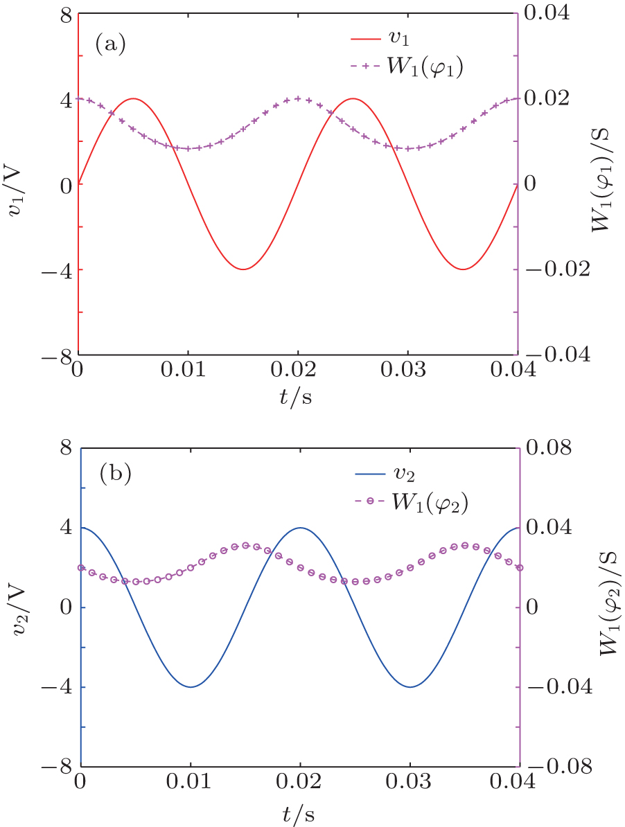 | Fig. 4. Time domain waveforms of the memductance of the decremental memristor under different excitation voltages. Vm = 4 V and f = 50 Hz. (a) Excitation voltage v1. (b) Excitation voltage v2. |
Figure 5 shows that the i– v curve of our memristor under sinusoidal excitation is a zero-crossing and frequency-dependent pinched hysteresis loop, which means that the memristor will turn into a linear resistor as the frequency increases. How does the frequency of the supply voltage affect the performance of the memristor? Do the other parameters in Eq. (3) have any effect on the memristor’ s i– v curve? We take the decremental memristor as an example and supply the voltage v2 to it. By assuming that the amplitude of the exciting voltage at the initial time (t = 0) is 0, i.e., v = v2(t)| t= 0 = 0, the following formula can be obtained:
 |
where ω = 2π f.
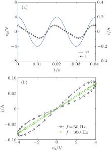
 | Fig. 5. The simulation results of the decremental memristor under the exciting voltage v2. (a) Time domain waveforms of the current when v2 (Vm = 4 V, f = 50 Hz) is supplied to the decremental memristor. (b) The i– v curves of decremental memristor with different frequencies. |
From Eqs. (4) and (5), the relationship between the current through and the voltage across the decremental memristor can be derived as
 |
As shown in Eq. (6), the current i is a double-valued function of the voltage v. What is more, due to i(v) = − i(− v), the i– v curve of the memristor must be odd symmetric with respect to the origin. Accordingly, for simplicity, the i– v curve within (0, T/4) and (3T/4, T) is discussed (i.e., the positive interval of v2). From Fig. 5(b) and the variation law of the decremental memristor’ s memductance, the i– v curve in (0, T/4) should be a concave curve, while the part in (3T/4, T) should be a convex curve. Note that the convexity or concavity of a curve can be determined by its second derivative. The second derivative of Eq. (6) can be calculated as follows:
 |
For the decremental memristor, there should be 

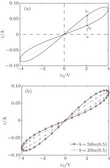
Figure 6 illustrates the analytical approach about the parameters’ effect on the memristor. As depicted in Fig. 6(a), for any two points on the i– v curve of the decremental memristor which have the same abscissa (the voltage), their position relationship can be described by the ratio of their ordinates (the current), i.e.,
 |
From Eq. (8), due to b < 0, one can see that λ will gradually close to 1 as b or ω increases. In other words, the decremental memristor will turn into a linear resistor if b or the frequency is too large, as shown in Figs. 5(b) and 6(b).
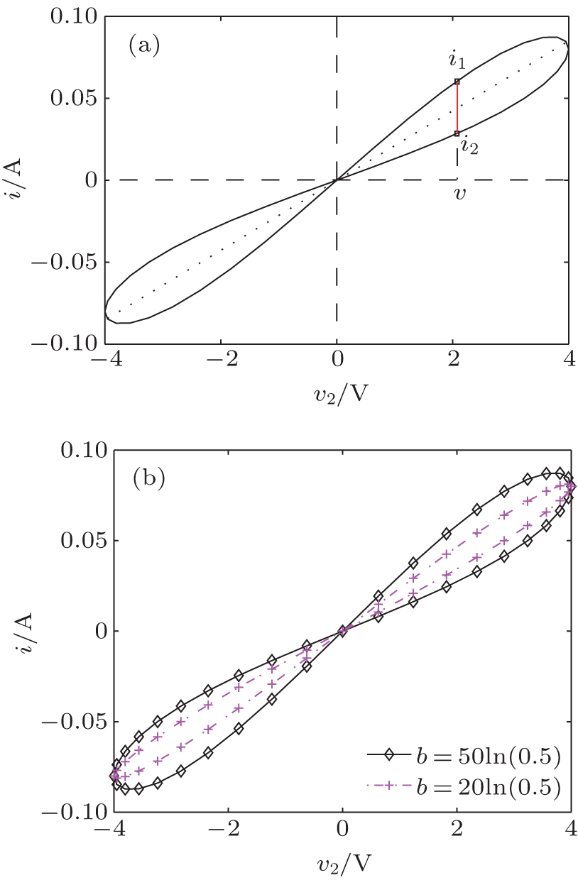 | Fig. 6. Schematic diagrams of the analytical approach about parameters’ effect on the memristor. (a) Position relationship of the selected two points. (b) The i– v curves of decremental memristor with different values of b when v2 is supplied to the decremental memristor. Here f = 50 Hz, and a = e. |
Above all, the model (3) possesses the features of the memristor and ensures that the variation law of its memristance never changes under different exciting voltages.
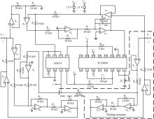
According to Eq. (6) and by considering that φ is the integral of the terminal voltage v, the floating emulator for the decremental memristor can be designed by a rational combination of the multiplication circuit, the integrated circuit, the adder circuit, the subtraction circuit, the exponential circuit, and the floating structures. The full schematic of the floating decremental memristor emulator is depicted in Fig. 7.
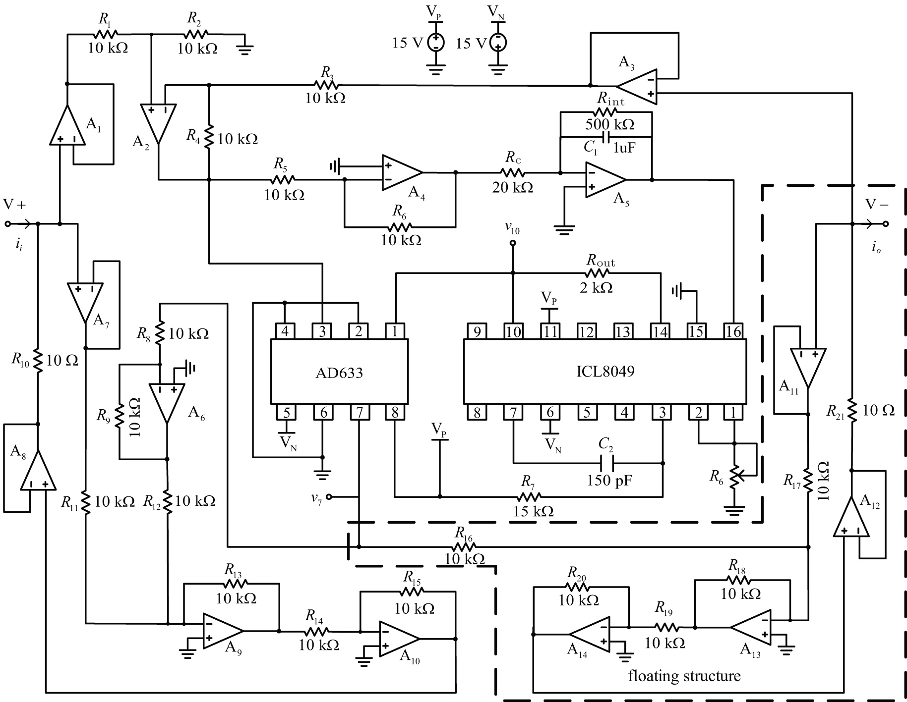 | Fig. 7. Full schematic of the floating decremental memristor emulator. |
The multiplication circuit is implemented by an analog multiplier AD633 whose output voltage v7 is one-tenth of the product of the ‘ 1 input voltage’ and ‘ 3 input voltage’ .
The output voltage of the operational amplifier AN is denoted by vAN, where N is a natural number. The subtraction circuit, which consists of A1, A2, and A3 is used to obtain the voltage across the memristor vin. The capacitor C1, A4, and A5 produce the flux φ by integrating vin.
The exponential circuit is implemented by a monolithic antilogarithmic amplifier ICL8049 and its output voltage can be approximately given by
 |
The function f(R6) is the scale factor which is a single-valued function of R6. By connecting the input to a precise 1 V supply and adjusting the potentiometer R6 for v10 = 1 V, one can obtain f(R6) = − ln(0.5).
As shown in Fig. 7, the floating structure of the input terminal of the emulator consists of A6, A7, A8, A9, and A10, while that of the output terminal is composed of A11, A12, A13, and A14. The resistor R10 is equal to R21. Note that the input currents of the operational amplifiers are so small that they can be ignored. Then, the following equations can be obtained:
 |
 |
 |
In the same way, the input current of the emulator can be given by
 |
According to the above analysis, the following equations (assuming that the initial voltage across the capacitor C1 is 0 V) can be derived:
 |
 |
 |
From Eqs. (9) and (14)– (16), one can obtain
 |
By comparing Eq. (17) with Eq. (6), the parameters of the proposed decremental memristor can be calculated as follows:
 |
From Eqs. (17) and (18), one can see that it is effective to use the designed circuit in Fig. 7 to implement the proposed decremental memristor. At the same time, the input current of the memristor emulator is equal to the output current, which means that the emulator is floating-ground. Moreover, this design of floating structure can be flexible enough to satisfy different demands for the current through the memristor (especially the demand for a larger current) simply by selecting different types of amplifiers to implement A8 (A12) and adjusting the resistor R10 (R21). For instance, if A8 and A12 are implemented by the high-voltage and high-current operation amplifiers, a larger input (output) current can be conveniently obtained. Furthermore, this design approach can also be used to improve other emulators with ground restriction. If the antilog amplifier ICL8049 in Fig. 7 is replaced by a multiplication circuit and an adder circuit, figure 7 will turn into a floating schematic of the emulator proposed in the Ref. [25].
In order to further verify the effectiveness of the floating memristor emulator, some experimental results are presented. In our experiment, the voltage probe Gwinstek GTP-151R is used to detect the input (output) terminal voltage to ground (v+ (v− )) and the output voltage of the ICL8049 (v10), and the differential probe Tektronix P5200A is used to detect the terminal voltage across the decremental memristor emulator vin. The current probe Tektronix A622 is used to detect the input (output) terminal current ii (io). The digital storage oscilloscope Gwinstek GDS-3254 is used to measure and capture the measured waveforms from the probes.
In addition, all the operation amplifiers shown in Fig. 7 except A8 and A12 are implemented by LF356. The A8 and A12 are implemented by the high-voltage and high-current operation amplifiers OPA551 to facilitate the measurements of the terminal current. The R10 and R21 are implemented by power resistors.
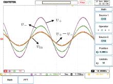
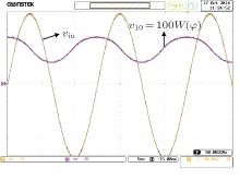
As shown in Fig. 8, channels 3 and 4 of the oscilloscope Gwinstek GDS-3254 are used to capture the input terminal voltage to ground (v+ ) and the output terminal voltage to ground (v− ), respectively. It can be observed that both of them are floating. The channel 1 is used to capture the voltage across the emulator (vin). The red line has displayed the result of ‘ CH3– CH4 (i.e., v+ − v− )’ by using the math subtract function in the oscilloscope Gwinstek GDS-3254, and it is in good agreement with vin. In other words, the emulator is working at the floating-ground situation and the voltage across the emulator is vin = v+ − v− = Vm sin(2π ft + π /2) in the experiment, where Vm = 4 V and f = 50 Hz.
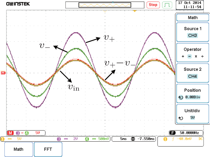 | Fig. 8. The measurements of the input terminal voltage to ground, the output terminal voltage to ground, and the voltage across the emulator. X-axis: 5 ms/div; Y-axis: 5 V/div for vin, 2 V/div for v+ , 500 mV/div for v− , 5 V/div for vM, 5 V/div for (v+ − v− ). |
By comparing Eq. (17) with Eq. (9), it can be observed that v10 = 10R10W(φ ) = 100W(φ ). Thus, the time-domain waveforms of v10 can be used as a substitute for W(φ ) to observe the variation law of the memductance. The experimental results about the variation of the memductance along the time are shown in Fig. 9, which agree very well with the analytical results in Fig. 4(b), i.e., v10 is monotonically decreasing (increasing) when the terminal voltage vin is positive (negative), and these prove that the emulator can represent a decremental memristor.
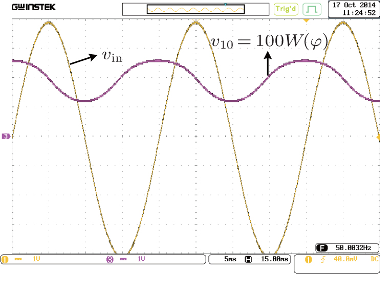 | Fig. 9. Variations of the memductance with time. X-axis: 5 ms/div; Y-axis: 1 V/div. |
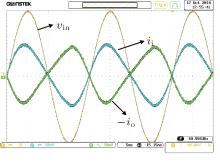
In order to observe the terminal current, channels 2 and 4 are used to capture the currents flowing in the input terminal and the output terminal of the emulator, respectively. As shown in Fig. 10, the current into the input terminal is consistent with the current from the output terminal, which proves the validity of the floating memristor emulator. The experimental results in Fig. 10 also agree very well with Fig. 5(a). Note that the input (output) currents’ peak has been approximated to 100 mA.
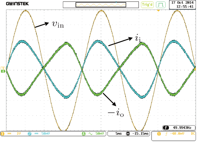 | Fig. 10. The time domain waveforms of the currents flowing into the input terminal and the output terminal of the emulator. X-axis: 5 ms/div; Y-axis: 1 V/div for vin, 50 mA/div for ii, 50 mA/div for io. |
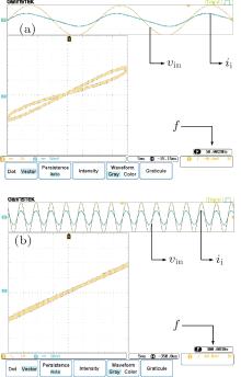
The i– v curves of the emulator in Fig. 11 show that the curve will tend to be a straight line as the excitation frequency increases.
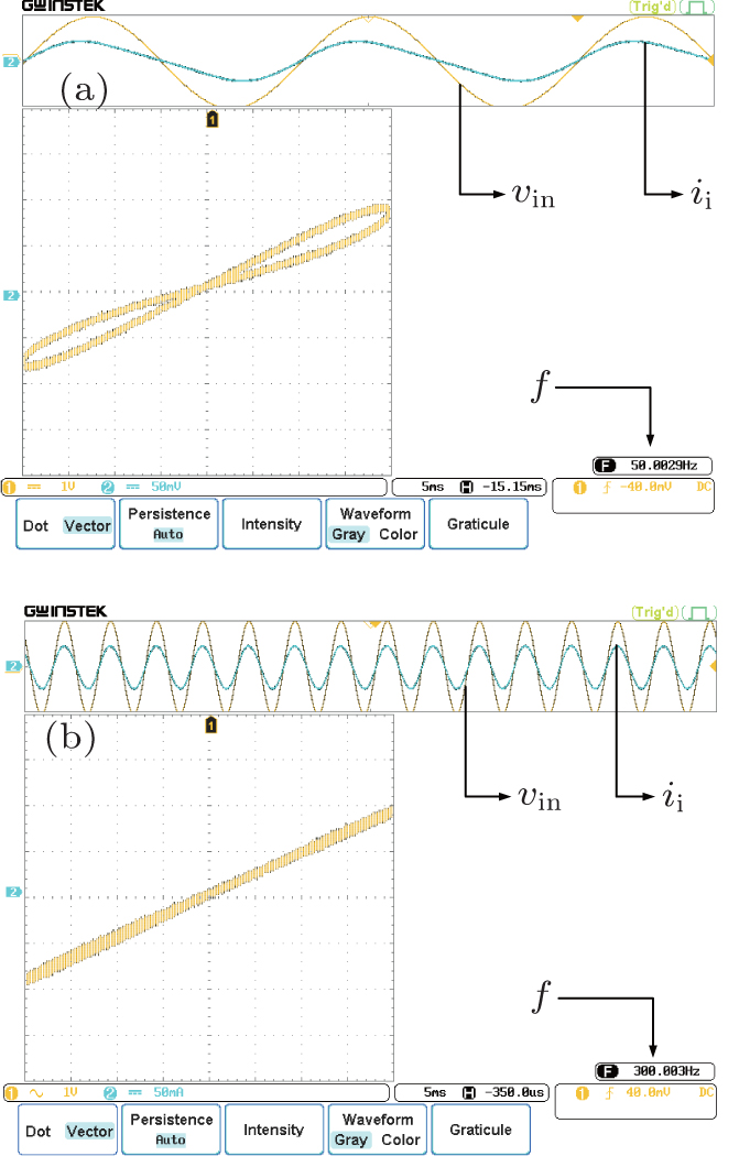 | Fig. 11. The i– v curves of the emulator: (a) f = 50 Hz, (b) f = 300 Hz. The horizontal axis represents vin, while the vertical axis represents ii. |
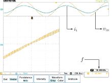
From Eq. (18), one can see that the value of b can be adjusted by the product of RcC1. Figure 12 shows that the i– v curve of the emulator is very close to a straight line when b is large enough.
 | Fig. 12. The i– v curves of the emulator when b is larger. The horizontal axis represents vin, while the vertical axis represents ii. Here f = 50 Hz, Rc = 50 kΩ , and C1 = 1 μ F. |
To sum up, the experimental results here are in agreement with the theoretical analysis. Therefore, the design scheme for a floating memristor emulator proposed here is effective.
This paper mainly focuses on two important matters in the research on the memristor: a model with a stable variation law of the memductance (memristance) under various excitation voltages and a floating hardware circuit that can emulate the features of the memristor and allow a larger input (output) current. The former is resolved by using the exponential function to improve the flux-controlled model. The latter is implemented by a rational combination of some off-the-shelf solid state devices. The experimental results are in good agreement with the theoretical analysis.
| 1 |
|
| 2 |
|
| 3 |
|
| 4 |
|
| 5 |
|
| 6 |
|
| 7 |
|
| 8 |
|
| 9 |
|
| 10 |
|
| 11 |
|
| 12 |
|
| 13 |
|
| 14 |
|
| 15 |
|
| 16 |
|
| 17 |
|
| 18 |
|
| 19 |
|
| 20 |
|
| 21 |
|
| 22 |
|
| 23 |
|
| 24 |
|
| 25 |
|
| 26 |
|
| 27 |
|
| 28 |
|
| 29 |
|
| 30 |
|
| 31 |
|
| 32 |
|
| 33 |
|
| 34 |
|
| 35 |
|
| 36 |
|