Coherent effects in Λ -type three-level systems have been studied extensively for many years. There are various phenomena associated with these systems, for example, coherent population trapping, ^[1] lasing without inversion, ^[2] stimulated Raman adiabatic passage, ^[3] and electromagnetically induced transparency (EIT).^{[4– 6]} Because of its wide applications in the fields of nonlinear optics and quantum storage, EIT has especially attracted a great deal of attention over the past two decades. Physically, EIT is explained as the result of quantum Fano interference, ^[7] where the destructive interference between two excitation pathways leads to the cancellation of the response at a particular frequency.

We first present a brief review of the previous studies on the dispersive properties of the EIT resonance. Xiao et al.^[8] measured the dispersion of EIT in rubidium atoms using a Mach– Zehnder (MZ) interferometer and homodyne detection. Somewhat differently, a heterodyne interferometer was employed by Muller et al.^[9] to investigate the parametric dispersion of the coupling field. Zhu and co-workers^[10] reported an experimental observation of large Kerr nonlinearity based on EIT, using frequency modulation spectroscopy to measure simultaneously the phase shift and the amplitude attenuation experienced by the probe laser.

Recently, we performed an investigation of the resonant stimulated Raman gain and loss spectra in the Rb atomic vapor, ^{[11, 12]} and measured the gain and loss of the probe beam in the presence of a coupling field. The main feature of the experiment is that the stimulated Raman spectrum is directly related to the EIT resonance. One particularly interesting result is that the concept of Raman gain can be employed to explain the phenomenon of EIT. We have also found that in a Doppler-broadened system, the gain and loss can co-exist, leading to the polarization interference between atoms of different velocities. As a result, there is a sharp transition from gain to loss as the probe field frequency is scanned when the coupling field is detuned.

In this paper, we study the absorption and dispersion in a Doppler-broadened Λ -type three-level system by stimulated Raman spectroscopy with homodyne detection. As is well known, the slowing of light in the EIT resonance is due to its steep dispersion.^[13] However, compared with the absorption, the dispersion of the EIT resonance is rarely measured directly. This is partly because it usually requires more sophisticated techniques, such as homodyne or heterodyne interferometry. The advantage of using stimulated Raman spectroscopy is that it has higher sensitivity and the EIT spectrum is Doppler-free, so a small signal with large noise can be observed. Moreover, based on the Kramers– Kronig (KK) relation, we derive a general model that provides a unified explanation of the absorption and dispersion spectra.

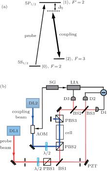
There are many ways to measure the dispersion properties of a medium. Here, we use the MZ interferometer together with homodyne detection because of its flexibility. The experimental setup is shown in Fig. 1. The probe and the coupling beams, which couple the D1 transition of Rb⁸⁵ from the hyperfine states 5S_1/2, F = 2 (| 0〉 ) and 5S_1/2, F = 3 (| 2〉 ) to the state 5P_1/2, F′ = 2 (| 1〉 ), respectively, are provided by two independent 795 nm diode lasers. An acousto-optic modulator (AOM) is employed to modulate the intensity of the coupling field by a signal generator (SG). The beams from the probe and the coupling lasers are horizontally and vertically polarized, respectively. A half-wave plate and a polarizing beam splitter (PBS1) are used to adjust the intensity of the probe beam. The probe beam is split into two paths by a beam splitter (BS1). In one path (the signal arm of the MZ interferometer), it is first combined with the coupling beam through a polarizing beam splitter PBS2 and then sent into the rubidium vapor cell at room temperature. The polarizing beam splitter PBS3 after the cell is used to filter out the coupling beam. The other path constitutes the reference arm of the interferometer, where the high reflecting mirror is mounted on a piezoceramic transducer. To make sure that the signal and the reference beams overlap, we monitor the interferometer fringes with a charge-coupled device camera. The small phase shift due the Rb⁸⁵ atoms in the cell is measured by homodyne detection with detectors D1 and D2, and the absorption coefficient α (ω ) is measured directly by detector D3.

Fig. 1.

	Figure Option ViewDownloadNew Window
	Fig. 1. (a) Energy level diagram. (b) Experimental setup (DL1 and DL2: diode lasers; AOM: acousto-optic modulator; λ /2: half-wave plate; PZT: mirror mounted on a piezoceramic transducer; BS: 50/50 beam splitter; PBS: polarizing beam splitter; D1, D2, and D3: photo detectors; SG: signal generator; LIA: lock-in amplifier).

The difference signal between the detectors D1 and D2 is given by

where L is the length of the cell, ϕ _Lo is the reference phase of the interferometer, E_s is the signal field after passing through the cell, E_Lo is the local oscillator field in the reference arm, and α (ω ) and β (ω ) are the absorption and dispersion coefficients, respectively. In our experiment, we set ϕ _Lo = π /2, then in the case of β (ω )L ≪ 1, we have

Finally, a lock-in amplifier (LIA) is used to demodulate the signals detected by the detectors. In our experiments, we lock the frequency of the coupling field while scanning that of the probe field, which has an intensity of about 2 μ W.

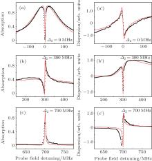
The results of our measurements are shown in Fig. 2. We consider three cases of the coupling field frequency: (i) exactly on resonance, (ii) detuned but still within the Doppler profile, and (iii) detuned far away from the Doppler profile. The black dots in Fig. 2 show the absorption (Figs. 2(a)– 2(c)) and dispersion (Figs. 2(a′ )– 2(c′ )) of the probe beam as a function of Δ ₁ when Δ ₂ = 0 MHz, 300 MHz, and 700 MHz for a coupling field intensity of 7 mW. Because the lock-in amplifier is used, only the absorption and dispersion induced by the coupling field could be measured, while the linear Doppler profile is eliminated from the spectrum. In addition, this technique increases the sensitivity of the measurements. When Δ ₂ = 0 MHz, we see a narrow transparent window at the center of the absorption profile (Fig. 2(a)). Correspondingly, the dispersion profile (Fig. 2(a′ )) exhibits an inverse dispersion shape. On the contrary, when the coupling field frequency is far away from the Doppler profile, we observe a sharp resonant absorption peak (Fig. 2(c)) with corresponding dispersion (Fig. 2(c′ )). The most interesting thing occurs when the detuning of the coupling field frequency is within the Doppler profile. Here, the absorption exhibits a sharp transition from gain to loss (Fig. 2(b)), so the absorption profile is dispersion-like. Correspondingly, the dispersion profile shows a sharp dip, which becomes absorption-like (Fig. 2(b′ )).

Fig. 2.

Figure Option ViewDownloadNew Window

Fig. 2. Experimentally measured (black dots) and theoretically calculated (red solid curves) absorption [(a)– (c)] and dispersion [(a′ )– (c′ )] curves of the probe beam as a function ofΔ 1 for a coupling field intensity of 7 mW when Δ 2 = 0 MHz [(a) and (a′ )], 300 MHz [(b) and (b′ )], and 700 MHz [(c) and (c′ )], respectively. Here, Γ 10 = 7.2 MHz, Γ 20 = 0.72 MHz, Γ = 5.75 MHz, γ = γ ′ = 0.12 MHz, and G2 = 20 MHz. In panels (a)– (c), the maximum of the absorption is normalized to 1.

In this section, we shall give a brief review of the theory of stimulated Raman spectroscopy, which has been discussed in detail in Ref. [11]. Let us consider a Λ -type three-level system (Fig. 1(a)), in which the states between | 0〉 and | 1〉 , and between | 1〉 and | 2〉 are coupled by dipolar transitions with resonant frequencies Ω ₁ and Ω ₂ and dipole moment matrix elements μ ₁ and μ ₂, respectively. A weak probe field (beam 1) of frequency ω ₁ is applied to the transition | 0〉 – | 1〉 , while a strong coupling field (beam 2) of frequency ω ₂ resonantly couples to the transition | 1〉 – | 2〉 to produce an EIT signal.

We are interested in how the coupling field affects the propagation of the probe beam. First, the coupling field can induce Raman coherence between | 0〉 and | 2〉 , which then interacts further with the coupling field and changes the amplitude of the probe field. Moreover, the coupling field can also cause a redistribution of the population, thus affecting the linear absorption of the probe beam. Therefore, the change in the atomic polarization due to the presence of the coupling field is given by

Here, the Raman coherence is given by

and the population redistribution is given by

where D = Γ ₁₀/(Δ ₂₂ + Γ ₂). The parameters in the above equations are defined as follows: Δ _i = Ω _i − ω _i are the detunings, G_i = μ _iE_i/ħ are the coupling coefficients, Γ _ij are the transverse relaxation rates between states | i〉 and | j〉 , γ (γ ′ ) is the relaxation rate from | 0〉 to | 2〉 (| 2〉 to | 0〉 ), and N is the atomic density.

In our experiment, we need to consider the effects of Doppler broadening. The total change of the atomic polarization is given by

Here, v is the atomic velocity, with , m is the mass of an atom, K is the Boltzmann constant, and T is the absolute temperature, while Δ P₁ (v) is given by Eq. (3) with Δ ₁ and Δ ₂ replaced by the Doppler-shift frequency detunings and , and k₁ and k₂ are the wave numbers. The imaginary and real parts of correspond to the absorption and dispersion of the spectrum, respectively. On the other hand, to obtain a better theoretical simulation of our experimental results, we need to include the excited state 5P_1/2, F′ = 3 (| 3〉 ). The involvement of this level can affect the population of the ground state, i.e., the term Δ ρ ₀₀ in Eq. (3). We use the following parameters to fit the experimental results: Γ ₁₀ = 7.2 MHz, Γ ₂₀ = 0.72 MHz, Γ = 5.75 MHz, γ = γ ′ = 0.12 MHz, and G₂ = 20 MHz. Here, we assume that γ = γ ′ because | 0〉 and | 2〉 are the hyperfine states. The red solid curves in Fig. 2. are the theoretical curves. The other parameters used in Fig. 2 are Δ ₂ = 0 MHz, 300 MHz, and 700 MHz. We see that the theoretical fits agree well with the experimental results.

In this section, we shall show that the dispersion and absorption are related by the Kramers– Kronig relation. We first review briefly this relation. As is well known, in linear optics, the KK relation relates the real part of the optical susceptibility to the imaginary part.^{[14, 15]} The underlying physics is the principle of causality. For the nonlinear case, the relation is no longer valid in a two-level atomic system if the saturation effect is included. However, by using multiple frequency arguments, it can still be satisfied in a nonlinear optical system.^{[16, 17]} Let χ (ω ) be the susceptibility of an optical system; if χ (ω ) has no poles in the lower half complex ω plane, then it can be shown that

where P denotes the Cauchy principal value. By decomposing χ (ω ) into the real and imaginary parts, i.e., χ (ω ) = χ ′ (ω ) − iχ ″ (ω ), we obtain

This is the KK relation.

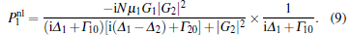
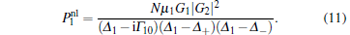
From Eq. (3), the polarization includes linear and nonlinear parts. Since the linear susceptibility satisfies the KK relation, we shall concentrate on the nonlinear polarization, which according to Eqs. (3) and (4) is given by

By solving for the pole in Eq. (9), i.e.,

we obtain

Here,

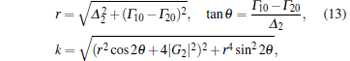
We note that for atoms with velocity v, the Doppler-shift frequency detuning is given by and . In our experiments, we measure the absorption and dispersion of the probe beam as a function of Δ ₁ (Fig. 2). To prove that they both satisfy the KK relation, we shall show that there are no poles in the lower half complex Δ ₁ plane. Let re^{− iθ} = Δ ₂ − i(Γ ₁₀ − Γ ₂₀) and ke^iφ = r²e^{− 2iθ} + 4| G₂| ², that is,

then equation (12) becomes

Moreover, from Eq. (14), we have

with

Finally, we obtain

which are the two corresponding terms in Eq. (15).

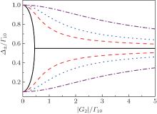
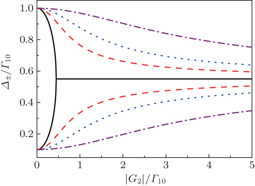
Figure 3 presents the dressed energies Δ _± /Γ ₁₀ as a function of coupling coefficient | G₂| /Γ ₁₀ with Γ ₂₀/Γ ₁₀ = 0.1 and Δ ₂/Γ ₁₀ = 0 (black solid curve), 1 (red dashed curve), 2 (blue dotted curve), and 5 (purple dashed-dotted curve). The upper curves are Im(Δ ₋ /Γ ₁₀), the lower ones are Im(Δ ₊ /Γ ₁₀), and the middle black solid line corresponds to ImΔ ₊ = ImΔ ₋ . Let us first consider the case when G₂ = 0. From Eq. (18), we have , and , therefore we obtain Δ ₊ = Δ ₂ + iΓ ₂₀ and Δ ₋ = iΓ ₁₀. Now let us consider limit G₂ → ∞ . In this case, we have α → 0, therefore, we obtain Δ _± → i(Γ ₁₀ + Γ ₂₀)/2 as G₂ → ∞ . We then calculate the derivative of the imaginary part of the dressed energies, and obtain

This shows that ImΔ ₊ increases with the increase of | G₂| . Therefore, as shown in Fig. 3, ImΔ ₊ increases from Γ ₂₀ to (Γ ₁₀ + Γ ₂₀)/2 as | G₂| changes from 0 to ∞ . Similarly, ImΔ ₋ decreases from Γ ₁₀to (Γ ₁₀ + Γ ₂₀)/2, as | G₂| increases. Since all poles of Δ ₁ for atoms of different velocities are in the upper half complex Δ ₁ plane, the KK relation, i.e.,

is satisfied in our case.

Fig. 3.

	Figure Option ViewDownloadNew Window
	Fig. 3. The dressed energies Δ ± = Γ 10 as a function of coupling coefficient | G2| = Γ 10 with Γ 20 = Γ 10 = 0.1, and Δ 2 = Γ 10 = 0 (black solid curve), 1 (red dashed curve), 2 (blue dotted curve), and 5 (purple dashed-dotted curve). The upper curves are Im(Δ − = Γ 10), the lower ones are Im(Δ + = Γ 10), and the middle black solid line corresponds to Im(Δ + ) = Im(Δ − ).

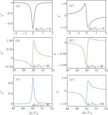
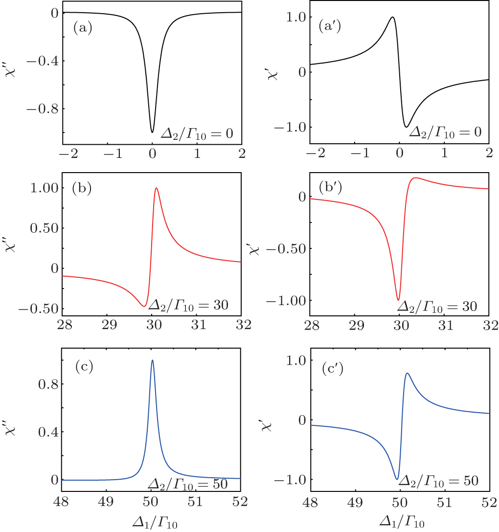
Now we turn to the experimental results shown in Fig. 2. First, the physical explanation of the absorption spectrum has already been given in our previous work.^[9] We then employ the KK relation to calculate the absorption and dispersion according to our experimental results by using Eqs. (8) and (9). For simplicity, we neglect the optical pumping effect and consider only the nonlinear part of the polarization. Figure 4 presents the numerical results for the imaginary (Figs. 4(a)– 4(c)) and real (Figs. 4(a′ )– 4(c′ )) parts of χ (Δ ₁/Γ ₁₀) in a Doppler-broadened Λ -type three-level system with the parameters Γ ₁₀/ku = 0.05, Γ ₂₀/Γ ₁₀ = 0.1, and G₂/Γ ₁₀ = 1. Here, Δ ₂/Γ ₁₀ is equal to 0, 30, and 50, respectively. In Fig. 4(a), the minimum of χ is normalized to − 1, while in Figs. 4(b) and 4(c), the maximum of χ is normalized to 1. As shown in Figs. 2 and 4, we obtain exactly the same results as in our experiment. One important feature of the KK relation is that a transformation takes place between the absorption and dispersion profiles. For example, when the coupling field frequency is far away from the Doppler profile, we observe a resonant absorption peak with a corresponding dispersion. On the other hand, when the detuning of the coupling field frequency is within the Doppler profile, the absorption profile is dispersion-like and the corresponding dispersion profile becomes absorption-like.

Fig. 4.

	Figure Option ViewDownloadNew Window
	Fig. 4. (a)– (c) Imaginary and (a′ )– (c′ ) real parts of χ (Δ 1/Γ 10) as a function of Δ 1/Γ 10 for Δ 2/Γ 10 = 0 [(a) and (a′ )], 30 [(b) and (b′ )], and 50 [(c) and (c′ )] withΓ 10/ku = 0.05, Γ 20/Γ 10 = 0.1, and G2/Γ 10 = 1. In panel (a), the minimum of χ ″ is normalized to − 1, while in panels (b) and (c), the maximum of χ ″ is normalized to 1.

We have measured the absorption and dispersion in a Doppler broadened Λ -type three-level system by resonant stimulated Raman gain and loss spectroscopy with homodyne detection. Through studying the dressed state energies of the system, it is found that the absorption and dispersion satisfy the KK relation. The absorption and dispersion spectra calculated by employing the KK-relation agree well with our experimental observations.