A Mach– Zehnder type atomic interferometer using the stimulated Raman transition^[7] utilizes the combination of π /2– π – π /2 Raman pulses of durations τ – 2τ – τ . The three pulses are separated by free evolving time T. Generally, the phase of the cold-atom interferometer is extracted from the atomic interference fringe, which is obtained by scanning the chirp rate α of the Raman lasers at a given interrogation time T. For the atoms free falling in the gravitational field, this chirp of the Raman frequency is also used to compensate the Doppler effect, if the direction of the Raman beams are in the vertical configuration. The interference fringe can be described as

where C is a contrast, and A is the ratio of offset.

Now, we introduce a new method of phase demodulation. We fix the chirp rate α , introduce a small positive resident Δ α ₀ = k_effg − α , then change the interrogation time T to step linearly one combined parameter Δ α ₀T², so that we can achieve a linear step of added phase. This means that the measured probability P_n is a function of the parameter , and the parameter T_n changes non-uniformly, here n is the measurement number. The measured probability P_n has the phase modulated cosine form (assuming T² as the time and Δ α ₀ as the frequency), and the modulating phase ϕ (T) is what we want to know. To demodulate the phase ϕ (T), we use a technique similar to phase demodulating for radio frequency by multiplying the fringe (after removing an estimated offset A₀) with the reference wave,

where ref_quphase and ref_inphase are the quadrature and the in-phase parts of the reference signal, respectively. The reference wave serves as the local oscillations. Then, the products of the multiplication are

After filtering by low-pass and band-stop filters (at the frequency of Δ α ₀ and its second harmonic), the two demodulated signal components P_qu and P_in have the form of the first term in Eq.  (3). Finally, we can calculate the demodulating phase ϕ (T) as a function of filtered P_qu and P_in. In this way, it is possible to track the phase larger than 2π . The result of arctan(P_in/P_qu) will give the phase ϕ (T) in the − π /2 to π /2 range. According to the sign of P_qu, we can add π to reach the range of − π /2 to 3π /2. Finally, by examining the gaps of 2π , we can add accumulated counts of 2π to each segment of the phase.

The measurement error in this demodulation method arises from two aspects: the filtering residual of the oscillations and the low-pass effect of filtering. By choosing the proper filter parameters, one can achieve more than 30  dB rejection at the oscillating frequency, which corresponds to 1  mrad in the phase error. The low-pass filter effect will lead to an error if the phase ϕ (T) signal has high frequency components, such as a step function, and the error also scales with the magnitudes of the high frequency components. If we measure close to time T where the step of the phase happens, with higher modulation frequency (larger Δ α ₀), we can increase the filter bandwidth and thus increase the time resolution.

Comparing with the method doing a localized cosine fit around any T with a chosen width and weight function, the demodulating method needs less calculation and is easy to treat a large phase shift.

Another utility of this method is to quickly obtain the absolute g value. When there is a second order phase drift ϕ (T) = Δ α ′ T², the absolute g can be obtained as (α + Δ α ₀ + Δ α ′ )/k_eff. However, when α in Eq.  (1) is larger than k_effg, the result of demodulating is indistinguishable with that of the smaller case, and the g should be (α − Δ α ₀ − Δ α ′ )/k_eff. Whether it is larger or smaller, the case can be verified by doing another linear scan of T² with the chirp rate equal to α + Δ α ₀ + Δ α ′ or α − Δ α ₀ − Δ α ′ . The right case should give the transition probability always at the minimal value of fringes (if as usually ϕ (T) is less than π /2).

During the process of the interference, the quantum axis is defined by the magnetic field produced by the coils. So there is a quadratic Zeeman phase shift in the total phase of the interference, which should be analyzed carefully. In this paper, we introduce three methods for the measurement of the quadratic Zeeman phase shift. The phase of the interferometer due to the quadratic Zeeman energy shift is written as

where Δ ω _Zeeman(t) = 2π KB(t)² is the quadratic Zeeman energy shift, K is the coefficient of the quadratic Zeeman effect, T_c is the circle time of each drop of atoms, and g_s(t) is the sensibility function of frequency shift at time t, which has the form

The quadratic Zeeman phase can be calculated once the magnetic field B(t) along the atom falling trajectory is measured. In this paper, we will also extract the quadratic Zeeman phase from the interference fringe.

Usually, reversing the direction of the two Raman lasers can form the interferometer with opposite effective wavevector of the Raman beams. By changing the sign of the chirp rate, the probabilities of atom transition from the initial state to another state are given by

where Δ α ₀ = k_effg − α , ϕ _dep is the phase term which changes sign when toggling the direction of the wavevector, and ϕ _indep is independent of the direction of the effective wavevector, which includes the quadratic Zeeman phase shift ϕ _Zeeman.

We use two methods to extract the quadratic Zeeman phase. The first one is called cosine fitting. For a given T and changing Δ α ₀, the phase shift can be obtained by fitting the fringes with a cosine function. The second one is called the phase demodulation as shown in Section 2. The phase demodulations of the probability of two effective Raman wavevector configurations are done independently. Lastly, averaging the phase shifts of the two opposite wavevectors, we can obtain the total independent terms for both fitting and demodulation methods.

To reach the same precision of phase shift estimation σ _{Δ ϕ} , the fringe fitting method needs shots of measurement, where σ _{ϕ , noise} is the equivalent phase noise in each shot. Considering the number of T of the final result N_point, the total shot of measurement is . On the other hand, the phase demodulation method takes the assumption that the phase shift has no quick change along T, thus one shot of T_n is contributing to adjacent N_filter points in the final result due to signal filtering. The benefit in the measurement time is 1/N_filter times for the same amount of result points and goal precision. In the cases where there are spikes or other fast changes in the phase shift, the filtering will spoil the signal, and introduce errors to adjacent points. We can overcome this by increasing the modulation frequency and making an adjustment of N_filter in the fast change regions to recover the detailed phase shifts.

We use the atomic interferometer in our lab^[25] to test the new phase demodulation method. The apparatus includes a cold rubidium 87 atom source and two phase locked lasers. About 10⁸ cold atoms are collected in a three-dimensional magnetic-optical trap (MOT), cooled by sub-Doppler cooling to a temperature of 5  μ K, and then released to free falling. The atoms are prepared in the first order Zeeman effect insensitive states, in this case, the m_F= 0 states, and the vertical velocity is selected by one π pulse of velocity sensitive Raman transition.

The Raman lasers are from the D2 line, which couple the two hyperfine structures of the 5²S_1/2 states by stimulated Raman transition. The Raman laser beams are emitted from one polarization-maintaining fiber and collimated by a lens system. The diameter of the Raman beams is 24  mm, the effective Rabi frequency is 41.7  kHz, and the duration of the π /2 pulse is around 6  μ s.

After three pulses of Raman lasers separated by time T, the interferometer signal, which is the population in the final state, is detected by collecting the fluorescence signal of the atoms scattering the detecting lasers.

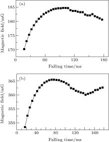
Firstly, the magnetic field in the interaction area can be measured with the spectral method. The magnetic field is generated by a pair of square coils around the system, which is used to maintain the axis of the quantum states in a residual magnetic background. The overall field is measured by the microwave spectrum^[25] of the cold atoms at different falling times. The result is shown in Fig.  1. For the differential measurement, the fields at the coil currents of 0.5  A and 1.0  A are measured independently.

Fig.  1.

	Figure Option ViewDownloadNew Window
	Fig.  1. The magnetic field strength as a function of the falling time: (a)  bias field current 0.5  A, (b) bias field current 1.0  A.

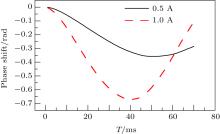
The magnetic field strength is interpolated before integrating to remove the effects of the limit measurement points. Then according to Eq.  (4), the corresponding quadratic Zeeman phase shift can be calculated by integration of the quadratic Zeeman frequency shift along the two interference trajectories. The numerical integration result shows that the overall peak phase error is about 700  mrad for the 1  A current case in Fig.  2.

Fig.  2.

	Figure Option ViewDownloadNew Window
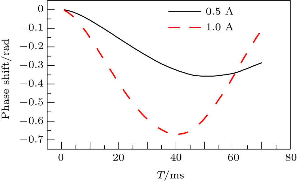	Fig.  2. The calculated quadratic Zeeman shift versus the interrogation time T.

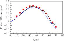
The interference fringes of pulse separation time T from 10  ms to 70  ms with 5  ms step are realized. The interference signal phase stepping is carried out by changing the chirping rate α of the Raman laser’ s frequency in a range where the change of α T² is about 4π . The cosine fitting results are shown as squares and triangles in Fig.  3. Usually, the fixed T method takes longer time and gives less result points.

Fig.  3.

	Figure Option ViewDownloadNew Window
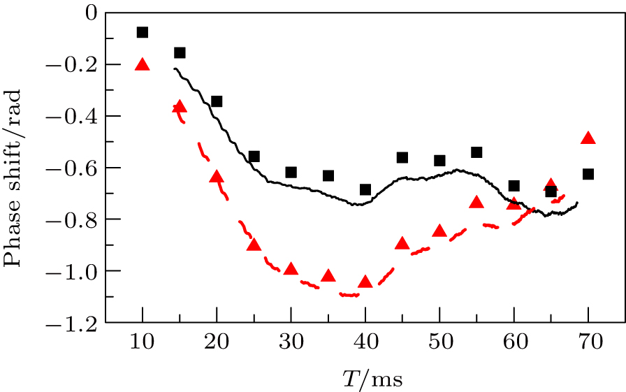	Fig.  3. The measured phase shift terms independent of the Raman wavevector versus the interrogation time T. The solid and dash lines are the scanning T2 phase demodulations with 0.5  A and 1.0  A bias fields, respectively; and the squares and triangles are the fixed T fringe fitting measurements with 0.5  A and 1.0  A bias fields, respectively.

To use the phase demodulation method, the atom transition probabilities are acquired for T² from 16  ms² to 4900  ms² with a step of 4  ms² (T = 4  ms to 70  ms with non-uniform steps). Using the reference wave of frequency Δ α ₀= 2π × 10  kHz to demodulate the probability signal as in Eq.  (3), we need to roughly estimate Δ α ₀, which needs to be sufficient for signal demodulating and filtering. In the demodulation, we use averages of 25 points and 13 points as filters to remove the residual harmonics at 10 kHz/s and 20 kHz/s. This method takes about one 25th of the time compared to the T fringe fitting method. The results are shown as lines in Fig.  3.

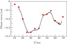
By comparing the results in Fig.  3 with the theoretical result (Fig.  2), it is obvious that there are other phase errors in the independent term. By only changing the current of the magnetic coils, these other effects may not change. This can be verified by comparing the differential phase shift. In Fig.  4, the differential quadratic Zeeman phase shift between 0.5 A bias field and 1 A bias field is matching the theoretically integrated result. The measurement errors are dominant by the vibration of ground and the response of the passive anti-vibration platform. For T = 70  ms, the fringe fitting method gives a standard error of 17  mrad and the phase demodulation method gives a standard error of 42  mrad. The results of the three methods are consistent within about 100  mrad, which proves that this new phase demodulation method is effective for rapidly extracting the phase of the atom interferometer.

Fig.  4.

	Figure Option ViewDownloadNew Window
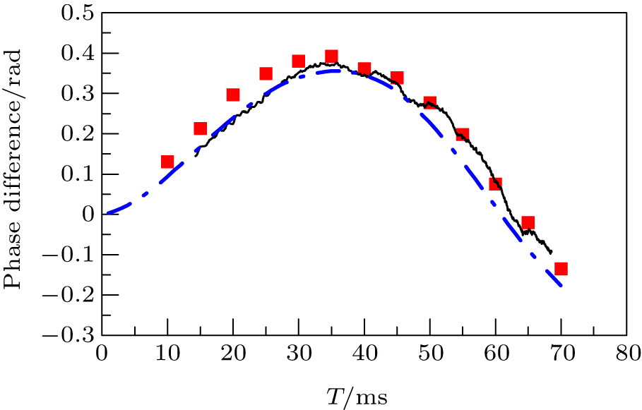	Fig.  4. Comparison of the results of differential phase shift between 0.5  A and 1.0  A bias fields. Line: scanning T2 phase demodulation; dash-dot line: calculated quadratic Zeeman shift; square: fixed T with fringe fitting measurement.

Other phase shifts independent of the wavevector of the Raman beams can be obtained by removing the calculated phase shift from the experiment phase shift, which is shown in Fig.  5. These phase shifts include those caused by the light shift and the frequency reference of the Raman lasers.

Fig.  5.

	Figure Option ViewDownloadNew Window
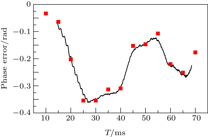	Fig.  5. Independent phase shifts other than the quadratic Zeeman shift. Line: scanning T2 phase demodulation; square: fixed T fringe fitting measurement.

We present a method of quickly mapping the phase shift of the atom interferometer as a function of the square of interrogation time (T²). Using non-uniformed steps of T but linear steps of one combined parameter Δ α ₀T², we can achieve a linear step of an added phase. Then the demodulation on the atom transition probability is used to extract the modulation phase.

The scan of T² and phase demodulation method has an advantage of more detailed mapping of the phase shift in smaller steps of T. But as the signal is obtained using demodulation, although with a notch filter, there are still some residual oscillations at the modulation frequency and its harmonics. The residual oscillations may limit the precision of this technique.

To demonstrate the techniques, the quadratic Zeeman shift is analyzed at different bias field currents. The results are compared with the fixed T fringe fitting measurements and the calculated quadratic Zeeman phase shift using direct magnetic field mapping. The results of the three methods are consistent.