


Performance characteristics of low-dissipative generalized Carnot cycles with external leakage losses*
[Huang Chuan-Kuna) , Guo Jun-Chengb)  , Chen Jin-Can
a) ]
, Chen Jin-Can]
|
|


†Corresponding author. E-mail: junchengguo@qq.com
Corresponding author. E-mail: jcchen@xmu.edu.cn
*Project supported by the Young Scientists Fund of the National Natural Science Foundation of China (Grant No. 11405032).
Under the assumption of low-dissipation, a unified model of generalized Carnot cycles with external leakage losses is established. Analytical expressions for the power output and efficiency are derived. The general performance characteristics between the power output and the efficiency are revealed. The maximum power output and efficiency are calculated. The lower and upper bounds of the efficiency at the maximum power output are determined. The results obtained here are universal and can be directly used to reveal the performance characteristics of different Carnot cycles, such as Carnot heat engines, Carnot-like heat engines, flux flow engines, gravitational engines, chemical engines, two-level quantum engines, etc.
Thermodynamic cycles are of great importance not only in theory but also in practice.[1– 8] The Carnot heat engine is one of the most important models in thermodynamics.[9, 10] Generalized Carnot cycles have been widely used in the various fields in physics.[11– 13] Investigations on the maximum power output of Carnot heat engines and other Carnot cycles and the efficiency at the maximum power output have attracted a great deal of attention during the last few decades and is a hot research topic.[14– 17] Recently, Esposito et al. established a new cycle model of Carnot heat engines on the basis of the weak dissipation assumption.[16] They proved that the efficiency of low-dissipative Carnot heat engines at the maximum power output is located between η C/2 and η C/(2 − η C), while the Curzon– Ahlborn efficiency[18]
The rest of the present paper is organized as follows. In Section 2, generalized Carnot cycles are briefly introduced and some examples are given. In Section 3, the model of low-dissipative generalized Carnot cycles with external leakage losses is proposed and the expressions of the power output and the efficiency are derived. In Section 4, the optimal relations between the power output and the efficiency are obtained. In Section 5, the maximum power outputs of cycles operated under different conditions are calculated and the bounds of the efficiency at the power output are determined. In Section 6, the performance characteristics related to the maximum efficiency are also discussed. In Section 7, the performance characteristics of the low-dissipative Carnot heat engine with heat leakage losses are directly obtained from the universal results. Finally, some important conclusions are drawn in Section 8.
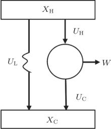
As is well known, heat engines operated in different temperature fields are able to produce useful work and thermodynamic cycles operated in other potential fields such as the chemical potential field, pressure field, gravitational field, quantum field, etc. are also able to obtain useful work. When thermodynamic cycles are operated in a potential field only including two reservoirs, which may be described by two parameters XH and XC (XH > XC), they are usually referred to as generalized Carnot cycles as shown in Fig. 1. Such cycles include four processes, where two processes exchange energy with two reservoirs and the other two processes do not exchange energy with two reservoirs, and can be taken as the models of some heat engines, [13– 18, 26– 28] flux flow engines, [29– 31] gravitational engines, chemical engines, [32– 35] two-level quantum engines, [36– 41] etc. For example, for a Carnot heat engine, XH and XC correspond to the temperatures TH and TC of high- and low-temperature heat reservoirs; for non-Carnot heat engines, [26– 28] which include the Otto cycle, [42, 43] Brayton cycle, [44– 46] Diesel cycle, [47, 48] and Atkinson cycle, [49, 50]XH and XC correspond to the highest temperature TH and lowest temperature TC of the working substance; for Carnot-like engines such as a gravitational engine, which may be regarded as an abstract model of hydropower stations or tidal power plants, XH and XC correspond to the height HH and HC of high- and low-gravitational potential energy reservoirs. For different types of engines, the parameters corresponding to XH and XC are listed in Table 1, where η r, g is the reversible efficiency of generalized Carnot cycles. Some signs in Table 1 are explained as follows. The F(S1, S2) is the total entropy change varying with the spin angular momenta Si = 〈 Ŝ z〉 (i = 1, 2), [51– 53]CH and CC are the heat capacities of the working substance during two heat exchange processes of non-Carnot heat engines, [26, 27, 41]Tj (j = 1, 2) are the initial temperatures of the working substance in two heat exchange processes, and “ + ” and “ − ” in signs “ ± ” correspond to the cases of j = 1 and 2, respectively. The reversible efficiencies η r, g of such heat engines and the efficiencies η r, m at the maximum work output[41] are listed in Table 2, where τ = TC/TH, ν = CP/CV, and f = 1/(1 + ν ). The pH = | a1| 2 and pC = | b1| 2 are the probabilities of two different superposed states in the eigenstate | ϕ 1(L)〉 , and 
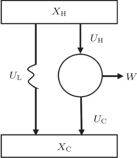 | Fig. 1. Schematic diagram of a generalized Carnot cycle with external leakage losses between two reservoirs. |
| Table 1. Parameters Xi (i = H, C) and Uir (i = H, C), and reversible efficiency η r, g of generalized Carnot cycles with different potential fields.[41] |
Under the low-dissipation assumption, [16] for an irreversible generalized Carnot cycle operated between two different potential energy reservoirs, the energies absorbed from the high-potential energy reservoir and released into the low-potential energy reservoir by the working substance per cycle can be expressed respectively as
 |
 |
where UHr and UCr, whose expressions are also listed in Table 1, are the exchange energies between the working substance and the two potential energy reservoirs when the reversible cycle is carried out, σ H and σ C are two parameters containing the concrete irreversibility, tH and tC are, respectively, the time durations in which the working substance contacts with the high- and low-potential energy reservoirs. This assumption means that compared with energy transfer times tH and tC, the relaxation time of the working substance in the cycle is very fast, and that, by ignoring complicated time-dependent terms due to the non-equilibrium between the reservoirs and the working substance, energy dissipations are expected to behave as σ H/tH and σ C/tC along high- and low-potential energy segments of the cycle. It is seen from Eqs. (1) and (2) that the cycle will return to reversibility when tH → ∞ and tC → ∞ . Compared with tH and tC, the times spent in two processes without energy exchange are further assumed to be negligible. Thus, the time spent in finishing one cycle may be approximately expressed as t = tH + tC.
Usually, the external leakage losses inevitably occur between two potential energy reservoirs and will affect the performance of the cycle. The external leakage losses per cycle UL shown in Fig. 1 may be simply described by
 |
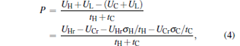
where uL is the rate of the external leakage losses from the high-potential energy reservoir to the low-potential energy reservoir. In general, uL is dependent on the energy reservoir and will have different values for different energy reservoirs. However, uL can be regarded as a constant for given energy reservoirs. Using Eqs. (1)– (3), we can derive the power output P and the efficiency η of the generalized Carnot cycle with the external leakage losses as
 |
 |
Using Eqs. (4) and (5), one can discuss the performance characteristics of low-dissipative generalized Carnot cycles with external leakage losses between the two reservoirs.
In order to obtain the optimal relations between the power output and the efficiency of low-dissipative generalized Carnot cycles with external leakage losses, we introduce the Lagrangian function
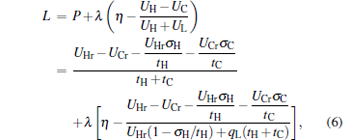 |
where λ is the Lagrangian multiplier. By using Eq. (6) and the Euler– Lagrange equations ∂ L/∂ tH = 0 and ∂ L/∂ tC = 0, an important relation
 |
is obtained. Equation (7) can be solved as
 |
where 
 |
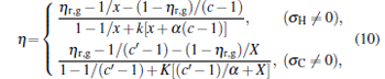 |
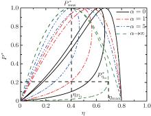
where η r, g= 1 − UCr/UHr, k = uLσ H/UHr, and K = uLσ C/UHr. By using Eqs. (9) and (10), the general characteristic curves of the power output varying with the efficiency can be generated with the help of a numerical calculation, as shown in Fig. 2, where the controlling parameter is x or X, P* = P/Pmax is the normalized power output, and the parabolic-shaped and loop-shaped curves correspond to the cases of k = 0 or K = 0, and k ≠ 0 or K ≠ 0, respectively. When 0 < α < ∞ , k = α k, and consequently, the first and second equations in Eq. (9) or (10) are equivalent to each other. When α = 0 or α → ∞ , both k and K may have the same values because they correspond to different curves, respectively.
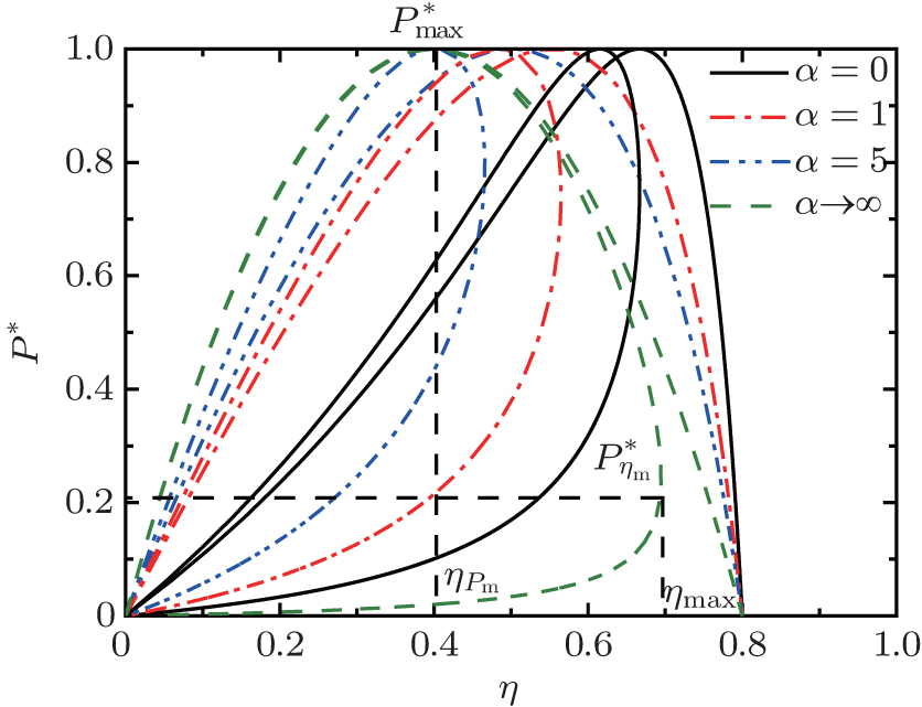 | Fig. 2. Curves of the dimensionless power output P* versus η for different values of α , where η r, g= 0.8, and k = 0 and 0.02. When α → ∞ , the value of K is chosen to be equal to that of k, respectively. |
It can be clearly seen from Fig. 2 that when the external leakage losses between two reservoirs are negligible, the η – P* characteristic curves are parabolic. The power output is equal to zero when the efficiency reaches the reversible efficiency η r, g. When the influence of external leakage losses between two reservoirs is considered, the η – P* characteristic curves become looped shapes. The maximum efficiency η max is smaller than η r, g, and the power output at the maximum efficiency is larger than zero. For a given value of k or K, the efficiency at the maximum power output increases with the decrease of α , and for a given value of α , the efficiency at the maximum power output with external leakage losses between two reservoirs is always smaller than that without external leakage losses. Figure 2 also shows that when the efficiency is smaller than η Pm, the power output of generalized Carnot cycles decreases with the decrease of the efficiency, and when the power output is smaller than 


It is significant to note that for some special values of α , some simple expressions of the power output and efficiency may be directly derived from Eqs. (9) and (10). For instance, when α → 0 and σ H is finite, the power output and the efficiency can be expressed as
 |
When α = 1, i.e., σ H = σ C, the power output and the efficiency are given by
 |
which correspond to the so-called symmetric dissipation.[16] When α → ∞ and σ C is finite, the power output and the efficiency can be obtained as
 |
From Eq. (9) and dP/dη = 0, it can be proved that when
 |
the power output attains its maximum, i.e.,
 |
and the corresponding efficiency is given by
 |
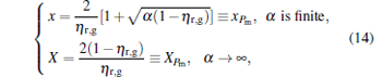
where

By using Eqs. (15) and (16), the 
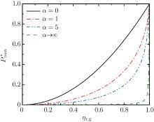
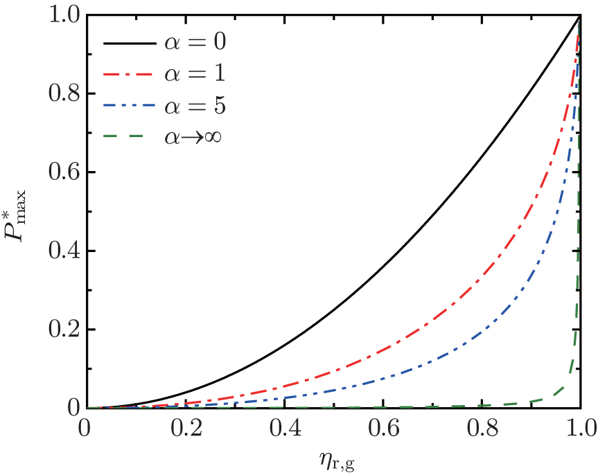 | Fig. 3. Curves of the maximum power output  |
Figure 3 shows that 

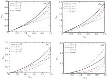
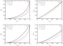
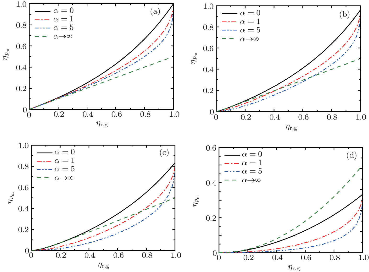 | Fig. 4. Variations of the efficiency at the maximum power output with reversible efficiency η r, g for different values of α and k, where (a) k = 0, (b) k = 0.01, (c) k = 0.05, and (d) k = 0.5. In panels (a)– (d), when α → ∞ , the value of K is chosen to be equal to that of k, respectively. |
Besides, for some special values of α , the expressions of the maximum power output and the corresponding efficiency can be obtained by using Eqs. (15) and (16). For example, when α → 0, the maximum power output and the corresponding efficiency can be simplified into
 |
 |
When α = 1, the maximum power output and the corresponding efficiency are derived as
 |
 |
When α → ∞ , the maximum power output and the corresponding efficiency are given by
 |
 |
It can be found from Fig. 2 that there exists not only a maximum power output but also a maximum efficiency for the generalized Carnot cycles with external leakage losses. According to Eq. (10) and dη /dP = 0, one can derive a relation as
 |
For general cases, we can obtain the values xη m and Xη m of x and X at the maximum efficiency by using Eq. (23) and the numerical calculation. For some special values of α , equation (23) is solvable. For example, when α = 0, we obtain
 |
where 
 |
 |
When α = 1, the solution is given by
 |
where 
 |
 |
For α → ∞ , from the second equation of Eq. (23), we derive
 |
where 
 |
 |
By using the above equations, the 
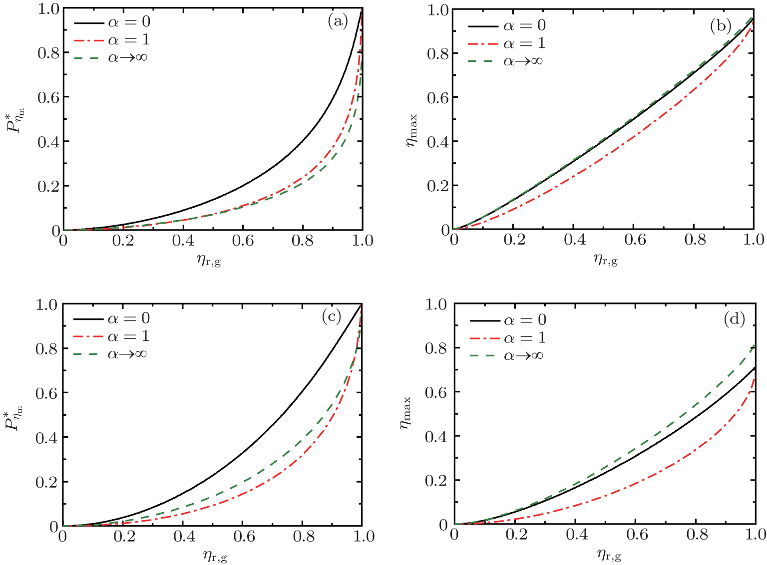 | Fig. 5. Variations of the maximum efficiency and the corresponding power output with reversible efficiency η r, g for different values of α and k: k = 0.01 ((a) and (b)) and k = 0.1 ((c) and (d)). In panels (a)– (d), when α → ∞ , the value of K is chosen to be equal to that of k, respectively. |
Figures 5(a) and 5(c) show that when k = K = 0.01 and k = K = 0.1, 


By using the results obtained above and Tables 1– 3, we can directly discuss the performance characteristics of various generalized Carnot cycles. For example, for a low-dissipative Carnot heat engine with heat leakage losses between the two heat reservoirs, we can obtain the performance characteristics of the heat engine as long as one chooses UH = QH, UC = QC, UL = QL, UHr = QHr = THΔ S, UCr = QCr = TCΔ S, and uL = qL, where Δ S is the entropy change of the working substance in the isothermal heat exchange process and qL is the rate of the heat leakage losses between two heat reservoirs. For some special values of α , we easily obtain the analytical expressions of the maximum power output Pmax and the corresponding efficiency η Pm, and the maximum efficiency η max and the corresponding power output Pη m of the low-dissipative Carnot heat engine with heat leakage losses, which are listed in Table 4, where kc = qLσ H/QHr, Kc = qLσ C/QHr, and η r, g= 1 − TC/TH ≡ η r. If the heat leakage losses between two heat reservoirs are negligible, the optimal relations between the power output and the efficiency can be further simplified into
 |
 |
 |
which are exactly the results obtained in Refs. [21] and [41]. The efficiency at the maximum power output is given by
 |
 |
 |
respectively, which are the results obtained in Ref. [16]. For other kinds of low-dissipative generalized Carnot cycles with external leakage losses, similar discussion may be carried out by using the above universal results and Tables 1– 3.
| Table 4. Expressions of some parameters of the low-dissipative Carnot heat engine with heat leakage losses for different values of α . |
Entropy production is often taken as an objective function in thermodynamic cycle optimizations.[54– 56] According to the above analyses, one can derive the entropy production per cycle for a low-dissipative Carnot heat engine as
 |
It is seen from Eq. (39) that when η = η r, then σ = 0. This means that if the maximum efficiency of a system can attain the Carnot efficiency, the state of the minimum entropy production corresponds to that of the maximum efficiency. If the maximum efficiency of a system is smaller than the Carnot efficiency, the minimum entropy production depends on both η and (QH + QL), and consequently, the state of the minimum entropy production is different from that of the maximum efficiency. Using Eq. (39), one can further obtain the relation between the entropy production rate and the power output as
 |
It is seen from Eq. (40) that the entropy production rate depends on both the efficiency and the power output. Thus, the state of the minimum entropy production rate is, in general, different from that of the maximum power output.
We have established the model of low-dissipative generalized Carnot cycles with external leakage losses, which may include several classes of typical engines, such as Carnot heat engines, Carnot-like engines, Carnot chemical engines, two-level quantum Carnot engines, etc. The expressions of the power output and efficiency are derived, and the optimal relations between them are discussed. The optimal operating regions are determined. The performance characteristics at the maximum power output and efficiency are analyzed. It is also expounded that like the efficiency and power output, the entropy production may be taken as an objective function of a thermodynamic system. There exist some certain relations between the entropy production and the efficiency and between the entropy production rate and the power output, but for general cases, the state of the minimum entropy production is different from that of the maximum efficiency and the state of the minimum entropy production rate is different from that of the maximum power output. The results obtained are universal, from which not only some important conclusions in the literature may be derived but also some novel results can be obtained.
| 1 |
|
| 2 |
|
| 3 |
|
| 4 |
|
| 5 |
|
| 6 |
|
| 7 |
|
| 8 |
|
| 9 |
|
| 10 |
|
| 11 |
|
| 12 |
|
| 13 |
|
| 14 |
|
| 15 |
|
| 16 |
|
| 17 |
|
| 18 |
|
| 19 |
|
| 20 |
|
| 21 |
|
| 22 |
|
| 23 |
|
| 24 |
|
| 25 |
|
| 26 |
|
| 27 |
|
| 28 |
|
| 29 |
|
| 30 |
|
| 31 |
|
| 32 |
|
| 33 |
|
| 34 |
|
| 35 |
|
| 36 |
|
| 37 |
|
| 38 |
|
| 39 |
|
| 40 |
|
| 41 |
|
| 42 |
|
| 43 |
|
| 44 |
|
| 45 |
|
| 46 |
|
| 47 |
|
| 48 |
|
| 49 |
|
| 50 |
|
| 51 |
|
| 52 |
|
| 53 |
|
| 54 |
|
| 55 |
|
| 56 |
|