
Optimized quantum random-walk search algorithm for multi-solution search*
[Zhang Yu-Chaoa), b) , Bao Wan-Sua), b)  , Wang Xiang
a), b) , Fu Xiang-Quna), b) ]
, Wang Xiang|
|


†Corresponding author. E-mail: 2010thzz@sina.com
*Project supported by the National Basic Research Program of China (Grant No. 2013CB338002).
This study investigates the multi-solution search of the optimized quantum random-walk search algorithm on the hypercube. Through generalizing the abstract search algorithm which is a general tool for analyzing the search on the graph to the multi-solution case, it can be applied to analyze the multi-solution case of quantum random-walk search on the graph directly. Thus, the computational complexity of the optimized quantum random-walk search algorithm for the multi-solution search is obtained. Through numerical simulations and analysis, we obtain a critical value of the proportion of solutions q. For a given q, we derive the relationship between the success rate of the algorithm and the number of iterations when q is no longer than the critical value.
The concepts of quantum computation and quantum computer[1] were proposed by Feynman in 1982. In 1985, Deutsch pointed out that the parallel quantum computation could be achieved by taking advantage of the coherent superposition of quantum states.[2] However, it was not until later when Shor’ s algorithm[3] and Grover’ s algorithm[4] were proposed that extensive attention into quantum computers and quantum algorithms was aroused.[5– 7] These greatly promoted the development of quantum computation and quantum communication technologies.
Essentially, Grover’ s algorithm is an exhaustive algorithm on the quantum computer. It solves the unsorted database search and achieves the quadratic speed-up compared with the classical algorithm. Although the Grover algorithm does not reach the obvious increase in speed compared with Shor’ s algorithm, the widely applicable search algorithm has also attracted people’ s attention. With the in-depth study, the efficiency of Grover’ s algorithm has been constantly improved, and it is more and more applied in practical problems. In 2001, Long proposed an improved Grover’ s algorithm with a success rate of 1 by replacing the phase inversion by phase rotation.[8] The Long algorithm[8] has proven to be optimal and the simplest by far.[9] In 2010, Wang et al. proposed a quantum algorithm for searching a target solution of fixed weight, which is more efficient to search for the NTRU private key.[10] In practice, the search space often contains a multi-solution. When Grover’ s algorithm is applied to the multi-solution search, the success rate of the algorithm has the potential to reduce. If the proportion of solutions is between 1/4 and 1/2, the success rate will reduce to 1/2. To solve this problem, there have been many improved algorithms proposed.[11– 13] Through altering the phase matching and the number of iterations, the success rate of the algorithm can be improved obviously. In Ref. [14], the multi-solution of Long’ s algorithm was also briefly mentioned. Moreover, the quantum deletion algorithms, [15, 16] which are related to the quantum search algorithm are presented. All the above studies make Grover’ s algorithm be used more and more widely, and promote the development of the quantum search algorithm.
In recent years, quantum random walks have attracted much attention.[17– 19] The quantum random walk is a generalization of random walk with the quantum mechanical, which can be used to design effective quantum algorithms.[20– 22] In 2003, Shenvi et al. proposed an algorithm based on quantum random walks (SKW algorithm), which is applied to the unsorted database search as Grover’ s algorithm.[23] The SKW algorithm is similar in many steps to the operation of Grover’ s algorithm. Both algorithms make use of the Grover diffusion operator. Both algorithms use an oracle which marks the target state with a phase of − 1, and both algorithms have a running time of 
However, the SKW algorithm was proposed only to search for one solution. Although numerical calculations suggest that it can also be used to search for a multi-solution, no related demonstrations and results have been presented. This is because when there is one solution, we use the method of geometric description to prove that the SKW algorithm is a rotation in the plane defined by the initial state and the final state, and the final state is composed primarily of the solution. When the number of solutions is larger than one, we cannot construct the final state properly to prove the algorithm by geometric description. In general, one solution is just a special case of multi-solution. Moreover, the optimized SKW algorithm can be generalized to the multi-solution case (Ref. [27]) based on the assumption that the SKW algorithm is applicable to the multi-solution case. Therefore, the research on the multi-solution case of the algorithm is meaningful and necessary whether on the algorithm itself or the follow-up research. In 2004, Ambainis et al. proposed an abstract search algorithm which is applied to search on the graph, and verified the correctness of the SKW algorithm with one solution.[29] In the same year, Szegedy showed how to analyze the multi-solution case for a different quantum walk algorithm, element distinctness.[30] These investigations provided ideas and possibilities for the study of the multi-solution case of the SKW algorithm and the optimized SKW algorithm.
This paper studies the multi-solution search of the optimized SKW algorithm. We first generalize the abstract search algorithm to the multi-solution case which is originally applied to search for one solution on the graph. Thus, it can be applied to analyze the multi-solution search of quantum random walk on the graph directly. Then, we obtain the computational complexity of the optimized SKW algorithm with multi-solution through the generalized abstract search algorithm. Using theoretical analysis and numerical simulations, we find that if the proportion of solutions q is small, the success rate of the algorithm and the number of iterations decrease with the increase of q. Finally, we obtain a critical value of q. When q is not larger than the critical value, for a given q, we derive the relationship between the success rate of the algorithm and the number of iterations.
The rest of this paper is organized as follows. In Section 2, we introduce the background. The optimized SKW algorithm with multi-solution is proposed in Section 3. In Section 4, we give the results of numerical simulations. The conclusion is given in Section 5.
The SKW algorithm is based on a quantum random walk on a hypercube. Let Cn = (Vn, En) denote the graph of the n-dimensional hypercube. The vertices Vn of the hypercube are labelled by binary, x = (x1, x2, … , xn), xi = {0, 1}. The Hamming weight of x is | x | . They are connected only if their Hamming distance is 1. The Hilbert space of the SKW algorithm is HCn ⊗ HVn where HVn is the 2n-dimensional Hilbert space representing the vertices, and HCn is the n-dimensional space associated with the quantum coin.
The operator of the SKW algorithm can be written as U' = SC' , where S is the shift operator
 |
where | ed〉 = | 0 · · · 010 · · · 0〉 corresponds to the edges originating from the given vertex, S performs a control transfer depending on the state of d. If the target is xtg, the coin operator can be written as
 |
where C0 is generally chosen as the Grover operator: − I + 2| SC〉 〈 SC| , and 
The initial state of the SKW algorithm is the equal superposition over all states 

The optimized SKW algorithm is based on the SKW algorithm, but quantum random walks occur on an (n + 1)-dimensional hypercube, p(x) = | x| mod 2 is denoted the parity bit of x. Then a map from the 2n-dimensional space to the 2n + 1-dimensional space can be built, x → x' = x | | p(x). After mapping, x corresponds to the vertices of an (n + 1)-dimensional hypercube, and the Hamming weights of them are even. Because x is one-to-one with x' , the oracle is capable of identifying the target after mapping.
The operator of the optimized SKW algorithm can be written as U' = S (C0 ⊗ I) SC' . Each iteration C' is only applied once, which is equivalent to calling the oracle once. The initial state is the equal superposition over coin space and the even vertice space | ψ 0(e)〉 . Applying the evolution operator U' to | ψ 0(e)〉 with 
The abstract search algorithm consists of two unitary transformations U1 and U2 and two states | ψ start〉 and | ψ good〉 . It requires the following properties. (i) U1 = I − 2 | ψ good〉 〈 ψ good| . (ii) U2 | ψ start〉 = | ψ start〉 , the amplitude of | ψ start〉 is real, and there is no other eigenvector with eigenvalue 1. (iii) U2 is described by a real unitary matrix.
The abstract search algorithm applies the unitary transformation (U2U1)T to the initial state with a proper T. The final state (U2U1)T | ψ start〉 has a sufficiently large inner product with | ψ good〉 . The main properties of abstract search algorithm will be given in the following.
Since U2 is a real unitary matrix, its non-± 1 eigenvalues come in pairs of complex conjugate numbers. Denote them by e± iθ 1, … , e± iθ m. Let θ min = min (θ 1, … , θ m) and U' = U2U1.
Lemma 1 Define the arc A as the set of eiθ for all real θ satisfying − θ min < θ < θ min. Then U' has at most two eigenvalues in A.
Let 

 |
Lemma 2 It is possible to select 


Lemma 3 The eigenvalues of U' in A are e± iα where
 |
Let | ω α 〉 and | ω − α 〉 be the two eigenvectors with eigenvalues eiα and e− iα , respectively. Define

and then, | ω start〉 is close to the starting state | ψ start〉 .
Lemma 4 Assume that α < θ min/2, and then
 |
Lemma 5 Assume that α < θ min/2. Let 
 |
According to the Lemmas of the abstract search algorithm, we can regard the algorithm being studied as an instance of the abstract search algorithm and then obtain the computational complexity of it.
The abstract search algorithm is proposed for the search of quantum random walks on the graph, but it applies to one solution. In Theorem 5 of Ref. [29], it is generalized to the case of two solutions. In this section, we will generalize the abstract search algorithm to the multi-solution case.
Lemma 6 The abstract search algorithm searching for four solutions v1, v2, v3, v4 is reduced to search for 

and s is the equal superposition over coin space.
Proof Assume v1 and v2 are two solutions and | ψ 〉 is the initial state, and U' is the operator of the algorithm. Then we can obtain the following relationship according to Claim 12 in Ref. [29]:
 |
where 

 |
where 
 |
Thus, the abstract search algorithm searching for four solutions reduces to searching for two superposition states. Lemma 6 is proved.
Lemma 7 The abstract search algorithm searching for four solutions v1, v2, v3, v4 is reduced to searching for 

Proof According to Eq. (7), the abstract search algorithm searching for two solutions v1 and v2 in space {v1, v2, … , vN} is reduced to searching for 

Similarly, searching for two solutions 


 |
If | s' i〉 is composed of elements in {v1, v2, … , vN} with the form of 

With Eq. (10), we have
 |
Combining Eqs. (9) and (11), we obtain the following relationship:
 |
where

Lemma 7 is proved.
Theorem 1 The abstract search algorithm searching for 2m solutions (2 < m < log 2N) is reduced to searching for s̃ 1, where 
Proof By induction, we proved the case of four solutions. If the inductive assumption case of 2m− 1 solutions is true, then we have
 |
where 
 |

which shows that the abstract search algorithm searching for 2m solutions is reduced to searching for s̄ 1 and s̄ 2.
On the other hand, the abstract search algorithm searching for two solutions s̄ 1 and s̄ 2 in space {s̄ 1, s̄ 2, … , s̄ M} is reduced to searching for 

thus
 |
When | s̄ i〉 is composed of elements in {v1, v2, … , vN} with the form of 

With Eq. (15), we have
 |
Combining Eqs. (14) and (16), we obtain
 |
where 
In this subsection, we generalize the abstract search algorithm to the case of multi-solution. Based on the above conclusion, we can use the abstract search algorithm to analyze the quantum random-walk search on the various graphs directly.
The relation between the optimized SKW algorithm and the SKW algorithm was given in Ref. [27]. Therefore, we only need to research the computational complexity of the SKW algorithm with multi-solution. The proof for one solution case is presented in Section 8 of Ref. [29]. The operation of the SKW algorithm can be written as U' = U(I − 2| s, xtg〉 〈 s, xtg| ) by the previous conclusion. We assume 2m solutions with 2 < m < log 2N. According to the Theorem 5 in Ref. [29], we only need to replace 
The eigenvalues and eigenvectors of U are already given in Ref. [31]. The quantum walk of the SKW algorithm stays in an 2n-imensional subspace spanned by 2n eigenvectors 


Theorem 2

Proof For the first part, because U' = U(I − 2| s, xtg〉 〈 s, xtg| ), we only show 


For the second part, assume | ω 0〉 is an eigenvector of eigenvalue 1 of U' in 
 |
This implies 

which in turn implies that | ω 0〉 is an eigenvector of eigenvalue 1 of U. Because 


Theorem 2 shows that the SKW algorithm with multi-solution starting in | ψ 〉 is restricted to a subspace 


Then, according to Lemma 3, we evaluate

which determines the computational complexity of the algorithm. Assuming 


Because 

Therefore, we only need to evaluate

which is the same as that in Section 8 of Ref. [29]. Therefore, 

Let | wα 〉 and | w− α 〉 be the two eigenvectors with eigenvalues eiα and e− iα , respectively, and define 

Finally, we show that measuring the final state 
according to Claim 10 in Ref. [29]. Furthermore,

according to Section 8 in Ref. [29], and 

Through the above proofs, we obtain the computational complexity of the SKW algorithm with multi-solution. According to Ref. [27], the computational complexity of the optimized SKW algorithm with multi-solution is also 
Through the abstract search algorithm, we can only obtain the computational complexity of the algorithm with multi-solution, but it does not involve the number of iterations. Therefore, we will further research the relationship between the success of the algorithm, the number of iterations, and the proportion of solutions by numerical simulations.
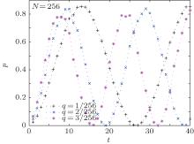
According to the conclusion of Subsection 3.2, if the proportion of solutions is small, the target will be obtained with a constant probability. Therefore, we first study the relationship between the success rate of the algorithm and the number of iterations with a small proportion of solutions. Figure 1 shows the relationship between the success rate of the algorithm and the number of iterations when the database size is N = 28. The proportions of solutions q = M/N are 1/256, 2/256, 3/256 respectively.
 | Fig. 1. Relationship between the success rate of the algorithm and the number of iterations for N = 28. The different lines show results for different values of q. |
It is known from Fig. 1 that the success rate of the algorithm changes periodically along with the number of iterations, and their relationship satisfies a trigonometric function approximately. If q is larger, the maximum success rate is smaller. This is consistent with the theoretical analysis. For one solution, the expression relating the success rate of the algorithm p and the number of iterations t is
where c is determined by n, and 1/c2 increases toward 1 with the increase of n. For multi-solution, considering the success rate of the algorithm p is equivalent to the proportion of solutions q when t = 0, we assume that the relationship satisfies
 |
By using curve fitting, ω and a are obtained. With n increasing, 

Then, we study the relationship between the success rate of the algorithm and the number of iterations when q is big enough.
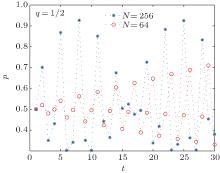
Figure 2 shows the success rate of the algorithm and the number of iterations for different databases with q = 1/2. Their relationship is no longer satisfying the previous function. Before the search, the success rate of the algorithm is 1/2 which is equivalent to the proportion of solutions q, and then it changes sharply along with the number of iterations. In practice, if q ≥ 1/2, we can directly obtain the target with a considerable probability without iterating the algorithm.
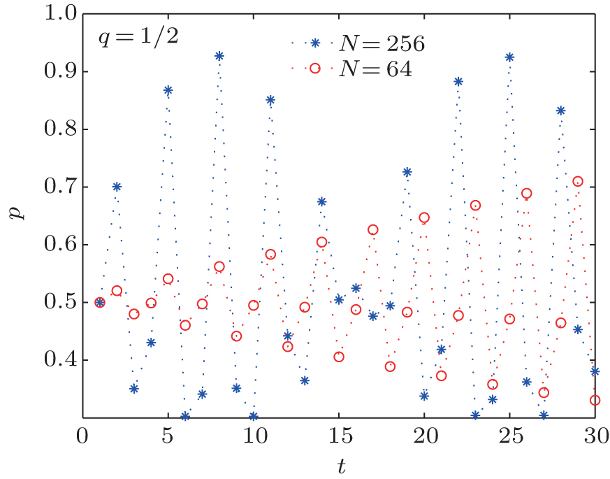 | Fig. 2. Relationship between the success rate of the algorithm and the number of iterations when q = 0.5. The circles line represents N = 64 and the asterisks line represents N = 256. |
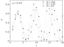
We obtain an approximate critical value of q by numerical simulations. Only if q ≤ 5/64, the success rate of the algorithm can reduce to 0 every time, as shown in Figs. 3 and 4. Therefore, we assume that the relationship curve still satisfies the form of Eq. (19).
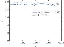
Finally, we study the relationship between the success rate of the algorithm and the proportion of solutions according to Eq. (19), as shown in Fig. 5. The solid line indicates the relationship for the optimized SKW algorithm when the number of iterations 
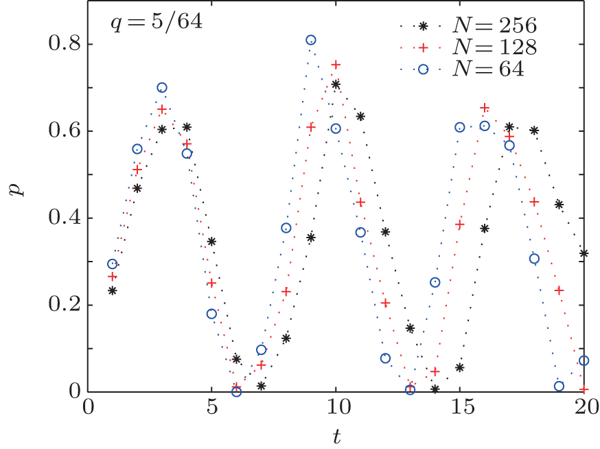 | Fig. 3. Relationship between the success rate of the algorithm and the number of iterations when q = 5/64. The different lines show results for different values of N. |
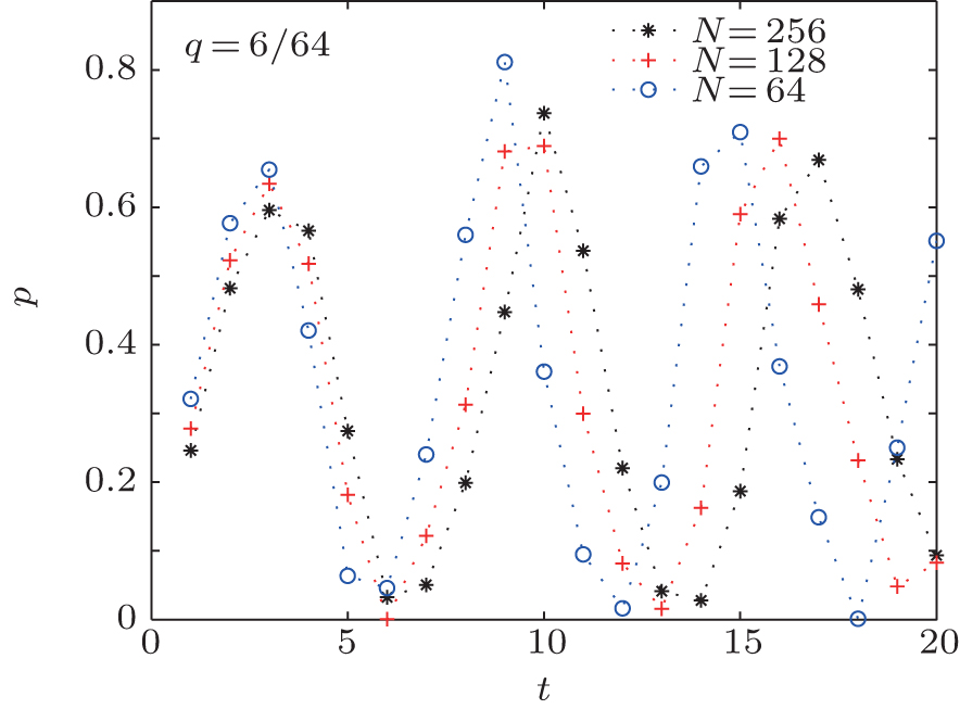 | Fig. 4. Relationship between the success rate of the algorithm and the number of iterations when q = 6/64. The different lines show results for different values of N. |
 | Fig. 5. Relationship between the success rate of the algorithm and the proportion of solutions for different algorithms. |
In this section, we simulate the relationship between the success rate of the optimized SKW algorithm and the number of iterations. We obtain a critical valve of the proportion of solutions. When q ≤ 5/64, the success rate of the algorithm, the number of iterations, and the proportion of solutions satisfy a quantitative relationship approximatively. When q > 5/64, the computational complexity of algorithm is still 
This paper investigates the multi-solution search of the optimized SKW algorithm. For the problem that the geometric description method cannot be applied to the multi-solution case directly, we first give the generalization of the abstract search algorithm for the multi-solution case. Then, we demonstrate that the computational complexity of the optimized SKW algorithm with multi-solution is 
When q > 5/64, the success rate is no longer periodically changing along with iterations, and the computational complexity of the algorithm is 
| 1 |
|
| 2 |
|
| 3 |
|
| 4 |
|
| 5 |
|
| 6 |
|
| 7 |
|
| 8 |
|
| 9 |
|
| 10 |
|
| 11 |
|
| 12 |
|
| 13 |
|
| 14 |
|
| 15 |
|
| 16 |
|
| 17 |
|
| 18 |
|
| 19 |
|
| 20 |
|
| 21 |
|
| 22 |
|
| 23 |
|
| 24 |
|
| 25 |
|
| 26 |
|
| 27 |
|
| 28 |
|
| 29 |
|
| 30 |
|
| 31 |
|