Exact solution of Heisenberg model with site-dependent exchange couplings and Dzyloshinsky–Moriya interaction
[Yang Li-Jun†a)  , Cao Jun-Peng
a), b) , Yang Wen-Lic), d) ]
, Cao Jun-Peng|
|


†Corresponding author. E-mail: chortley@iphy.ac.cn
*Project supported by the National Natural Science Foundation of China (Grant Nos. 11174335, 11375141, 11374334, and 11434013) and the National Program for Basic Research of China and the Fund from the Chinese Academy of Sciences.
We propose an integrable spin-1/2 Heisenberg model where the exchange couplings and Dzyloshinky–Moriya interactions are dependent on the sites. By employing the quantum inverse scattering method, we obtain the eigenvalues and the Bethe ansatz equation of the system with the periodic boundary condition. Furthermore, we obtain the exact solution and study the boundary effect of the system with the anti-periodic boundary condition via the off-diagonal Bethe ansatz. The operator identities of the transfer matrix at the inhomogeneous points are proved at the operator level. We construct the T– Q relation based on them. From which, we obtain the energy spectrum of the system. The corresponding eigenstates are also constructed. We find an interesting coherence state that is induced by the topological boundary.
Quantum integrable systems have attracted considerable interest because they can provide an exact insight into one-dimensional strongly correlated systems. Based on Yang’ s[1, 2] and Baxter’ s[3, 4] pioneering works, the Leningrad group proposed the quantum inverse scattering method (QISM) or the algebraic Bethe ansatz method[5– 9] for integrable systems with the periodic boundary condition (PBC). Later, this method was generalized to the open boundary cases.[10– 12] In the past several decades, the QISM has become one of the most powerful methods in solving the spectrum problem of integrable systems. In particular, the development of the nested algebraic Bethe ansatz[13– 16] enables one to diagonalize the multicomponent integrable models in a systematic way. However, the QISM fails when considering the anti-periodic boundary condition (APBC) because the particle number is not conserved and the U(1) symmetry is broken in this case. The APBC is physically interesting because it is related to the topological properties of the matter, with Jordan– Wigner transformation, it describes a p-wave Josephson junction in a spinless Luttinger liquid. For example, the APBC in the XX spin chain corresponds to a boundary coupling term of 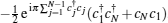

The Dzyaloshinsky– Moriya interaction (DMI)[23– 25]HDM = D· (S × S) is an antisymmetric spin-spin interaction which plays an essential role in various fields.[26– 29] The historical study of the Hamiltonian[30] of the Heisenberg model with the DMI is

where J is the exchange integral, Δ is the anisotropic parameter, D is the Dzyaloshinsky vector, and 
In this paper, we propose an integrable Heisenberg model with exchange couplings and DMI that are dependent on the sites. (In the following we call them the site-dependent exchange couplings and DMI.) We obtain exact solutions, including the energy spectrum and eigenstates of the system with different boundary conditions. The rest of this paper is organized as follows. In Section 2, we introduce the Hamiltonian and the rotation transformation which is essential in understanding the physics. In Section 3, we use the QISM to solve the Hamiltonian with the PBC. In Section 4, the ODBA is used to study the system with the APBC and we find a coherence reference state that is induced by the topological boundary. Our concluding remarks are discussed in Section 5.
We consider a one-dimensional Heisenberg model with the site-dependent exchange couplings and DMI. The Hamiltonian is
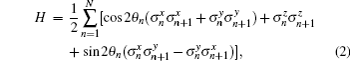
where N is the length of the system, σ α (α = x, y, z) is the 2 × 2 Pauli matrix, and {θ n, n = 1, … , N} are arbitrary site-dependent parameters, which are real to ensure the hermiticity of the Hamiltonian. When all of the site-dependent parameters {θ n} are equal to a constant, the system is reduced to the Hamiltonian (52) up to scaling factor.
We first introduce a rotation of the spins in the x– y plane with the transformation matrix

which is a 3 × 3 orthogonal matrix and satisfies U (θ n)TU (θ n) = id, U (θ n)T = U (− θ n) (T means the transposition). We can easily derive the following relations,
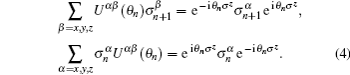
Under the transformation (3), the Hamiltonian (2) can be expressed as

Furthermore, we define

which means that we rotate each of the spins at site n with an angle 


Therefore, if 
In this section we show the integrability of the Hamiltonian (2) with the PBC. The R-matrix of the system is R0, n(u) = u + P0, n, where u is the spectral parameter and 

Below we list some important properties of the R-matrix,


where ϕ (u) = u2 − 1, Tj is the transposition in the space j and 

The Lax operator is defined as L0, n(u) = R0, n(u). Considering two Lax operators L0, n(u) and L0′ , n(ν ) with the same quantum space Vn and different auxiliary spaces V0 and V0′ , the product of L0, n(u) and L0′ , n(ν ) acts in the space Vn ⊗ V0 ⊗ V0′ and satisfies the Yang– Baxter equation (YBE)

which defines the underlying algebraic structure and is the cornerstone of solving the quantum integrable models. We consider a constant matrix 

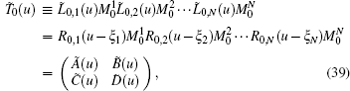
Define the monodromy matrix T0(u) as

which is a matrix in the auxiliary space V0 with its matrix elements being the operators acting on the quantum spaces. The transfer matrix is the trace of the monodromy matrix in the auxiliary space, i.e. t(u) = tr0T0(u). Obviously,

From Eqs. (16) and (18), we can prove that the monodromy matrix T0(u) satisfies the YBE

Left multiplying Eq. (19) with 

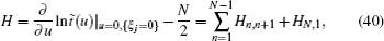
which means that the transfer matrices with different spectral parameters are mutually commutative. In such a sense, the transfer matrix serves as a generating functional of conserved quantities and ensures the integrability of the system. The Hamiltonian (2) is the first derivative of the logarithm of the transfer matrix

We denote the monodromy matrix as

From the YBE (19), the elements of the monodromy matrix satisfy the following commutation relations


We define the vacuum state of the system as

where | ↑ 〉 n is the spin up state of site n. The monodromy matrix T0(u) acting on the vacuum state gives

We see that the elements A(u) and D(u) acting on the vacuum state give the eigenvalues a(u) and d(u), respectively. The element C(u) acting on the vacuum state is zero and B(u) is the spin flipping operator, which are used to generate the eigenstates of the system.
Assume that the eigenstate of the system takes the form of

where {μ j, j = 1, … , M} are the Bethe roots and M is the number of flipped spins. With the notation (22), the transfer matrix is

Acting t(u) on the Bethe state (29), we should exchange the positions of A(u), D(u) and {B(μ j)} until A(u) and D(u) arrive at vacuum state. Repeat using the commutation relations (24) and (25), we then obtain


With the help of the commutation relations (31) and (32), the transfer matrix acting on the assumed Bethe state gives

where the eigenvalue term Λ (u) is

and the “ unwanted term” Λ j(u) is

If all of the unwanted terms {Λ j(u)} are zero, then the assumed Bethe state (29) is indeed the eigenstate of the transfer matrix, which requires that the Bethe roots {μ j} should satisfy the following Bethe ansatz equation (BAE),

For convenience, we put μ j = λ j − 1/2 and the BAE becomes
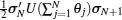
The eigenvalue of the Hamiltonian is

Now we consider the Hamiltonian (2) with the APBC, i.e. 
where {ξ j, j = 1, … , N} are the inhomogeneous parameters and à (u), B̃ (u), C̃ (u), D̃ (u) also satisfy the commutation relations (23)– (26). The corresponding transfer matrix is 
with the boundary relation

We first consider the effect of the boundary Eq. (41) and introduce a global rotation

We define

and then we have

With the global transformation (42) on each spin, the couplings in the bulk become 
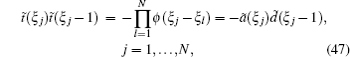
Due to the APBC, the state (27) is no longer a reference state of the system and the QISM does not work. We adopt the ODBA developed in Ref. [17] to solve the problem. The main idea of the ODBA is as follows. First we should find the operator production identities of the transfer matrix. Based on these identities, we can construct the inhomogeneous T– Q relation. From which we can obtain the eigenvalues and eigenstates of the transfer matrix and the Bethe ansatz equations. In order to obtain the operator identity, we evaluate the transfer matrix t̃ (u) at the point ξ j,
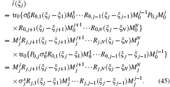
From Eq. (45), we see that t̃ (ξ j) is a reduced monodromy matrix by treating the j-th quantum space as the auxiliary space. The transfer matrix t̃ (u) at another point ξ j − 1 reads

In the derivations, we have used the crossing relation (10) of the R-matrix and 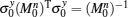
where

Correspondingly, the eigenvalues Λ ̃ (u) of the transfer matrix t̃ (u) should satisfy the functional relation

We note that the eigenvalue Λ ̃ (u) is a polynomial with degree N − 1, which can be completely determined by the N identities [Eq. (49)] of {Λ ̃ (u)}.
Based on Eq. (49), we parameterize the eigenvalue of the transfer matrix as

where ã (u) and d̃ (u) are defined in Eq. (48), the function Q̃ (u) is

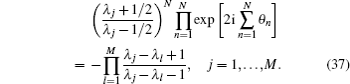
Notice that d(ξ j) = a(ξ j − 1) = 0, the ansatz equation (50) satisfies Eq. (49) automatically. As the eigenvalue of the transfer matrix is a polynomial, the residual of Eq. (50) must be zero, which gives the constraint of the values of the Bethe roots 

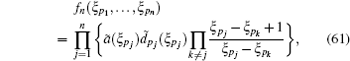
where 

We find that the site-dependent parameters {θ j} do not enter the BAE and the eigenvalue, which means that the effects of the site-dependent coupling is canceled by the APBC and is consistent with the analysis in Section 4.
We introduce the state | 0〉 with all of the spins up and its dual state 〈 0| ,

the elements of the monodromy matrix T̃ 0(u) that act on them are

where ã (u) and d̃ (u) are given by Eq. (48). Now we introduce the left and right states parameterized by the N inhomogeneous parameters {ξ j},


It is easy to prove that equations (56) and (57) are eigenstates of D̃ (u) that


The orthogonal relation between the left state and the right state is

where
with f0 = 〈 0| 0〉 = 1. The function d̃ l(u) is defined as

Thus the left/right states in Eq. (56)/Eq. (57) form a 2N-dimensional orthogonal left/right basis of the dual/the Hilbert space, and any left/right state can be decomposed as a unique combination of these basis.
Since the left states {〈 ξ p1, … , ξ pn| , n = 0, … , N, 1 ≤ p1 < p2 < … < pn ≤ N} given by Eq. (56) form a basis of the dual Hilbert space, the left eigenstate 〈 Ψ | can be expressed as

The orthogonal relation Eq. (60) allows us to determine the coefficientχ n (ξ p1, … , ξ pn) as

where Fn(ξ p1, … , ξ pn) is defined as

with F0 = 〈 Ψ | 0〉 = 1.
As 〈 Ψ | is an eigenstate of the transfer matrix t̃ (u), i.e., 〈 Ψ | t̃ (u) = 〈 Ψ | Λ ̃ (u), with Λ ̃ (u) given by Eq. (50), we can obtain the following relation by considering the quantity 〈 Ψ | t̃ (ξ pn+ 1)| ξ p1, … , ξ pn〉 ,

We consider the following Bethe state

where {λ j| j = 1, … , N} are the Bethe roots of the BAE (52) and | Ω ; {ξ j}〉 is a generalized reference state to be determined so that the condition (66) is fulfilled. For an eigenvalue Λ ̃ (u) given by the T– Q relation (50), its value at the inhomogeneous point ξ j takes

thus from 〈 ξ p1, … , ξ pn| λ 1, … , λ N〉 = Fn(ξ p1, … , ξ pn) we can prove that

We propose the following ansatz for the reference state | Ω ; {ξ j}〉

where the operator B̃ − is defined as

From the definition of the monodromy matrix T̃ (u), we can find the explicit expression of the operator B̃ − as

To prove that | Ω ; {ξ j}〉 given by Eq. (70) indeed satisfies the relation (66), we introduce the inner product

with g0 = 〈 0| 0〉 = 1. We can derive the following recursive relation for gn({ξ j}| {uα })

Define

the initial condition of ḡ n({ξ pj}) is ḡ 0 = 1. Thus, with the recursive relation (74) of gn({ξ j}| {uα }) and the following identity

we can derive the recursive relation of ḡ n({ξ j}),
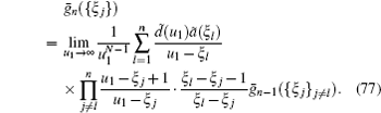
which determines the functions {ḡ n({ξ j})| n = 0, … , N} as

By substituting Eq. (78) into Eq. (75), we find that the state | Ω ; {ξ j}〉 given by Eq. (70) indeed satisfies the relation (66). In the homogeneous limit {ξ j → 0}, the reference state (70) becomes

This implies that the homogeneous limit of the Bethe state (67) with the reference state (70) gives rise to the eigenstate of the corresponding homogeneous transfer matrix, which provides that the parameters {λ j| j = 1, … , N} satisfy the BAE (52).
In summary, we proposed an integrable spin-1/2 Heisenberg model with site-dependent exchange coupling and DM interaction. We studied the system with different boundary conditions. By employing the QISM method, we obtained the eigenvalues and the Bethe ansatz equation of the system with PBC. The site-dependent parameters enter the BAE, thus affecting the eigenvalues and physics of the system. We also obtained the exact solution of the system with APBC and studied the boundary effect. The operator identities of the transfer matrix at the inhomogeneous points are proven at the operator level. We constructed the T– Q relation based on them. From it, we obtained the energy spectrum of the Hamiltonian. The corresponding eigenstates are also constructed. We find that due to the topological nature of APBC, the reference state is a perfect coherence state, which is very different from that of PBC, where the reference state is a direct product state.
| 1 |
|
| 2 |
|
| 3 |
|
| 4 |
|
| 5 |
|
| 6 |
|
| 7 |
|
| 8 |
|
| 9 |
|
| 10 |
|
| 11 |
|
| 12 |
|
| 13 |
|
| 14 |
|
| 15 |
|
| 16 |
|
| 17 |
|
| 18 |
|
| 19 |
|
| 20 |
|
| 21 |
|
| 22 |
|
| 23 |
|
| 24 |
|
| 25 |
|
| 26 |
|
| 27 |
|
| 28 |
|
| 29 |
|
| 30 |
|