Entanglement, an important trait in quantum mechanics, has become a key resource for many quantum processes.^[1] Entanglement can be experimentally prepared and manipulated in microscopic systems, such as photons, ions, and atoms.^[2] However, it is not yet completely clear to what extent quantum mechanics applies to macroscopic objects. Quantum phenomena such as entanglement generally do not appear in the macroscopic world due to environment-induced decoherence, which is thought to be the main cause that reduces any quantum superposition to a classical statistical mixture.^[3] Nonetheless, with the spectacular level of experimental advancements, it has been possible to see macroscopic quantum superpositions.^[4]

Cavity optomechanical systems have become important candidates for exploring what extent of quantum entanglement we can obtain at the macroscopic level^{[5– 13]} due to the rapid progress of nanotechnology. The simplest scheme capable of generating stationary optomechanical entanglement is studied in a typical optomechanical setup, ^[14] where the entanglement between the cavity and the movable mirror is remarkable for its simplicity and robustness against temperature. In recent years, various schemes to generate bipartite entanglements have been proposed, such as the field– mirror entanglement, ^{[15– 20]} and the mirror– mirror entanglement.^{[21– 24]} These studies show that entanglement can be influenced by the factors of the cavity optomechanical system such as the intensity of incident laser and the cavity– pump field detuning. In fact, entangled optomechanical systems have potential profitable applications in realizing quantum communication networks, in which the mechanical modes play the vital role of local nodes where quantum information can be stored and retrieved, and optical modes carry the information between the nodes. This allows the implementation of continuous variable (CV) quantum teleportation, ^{[25, 26]} quantum telecloning, ^[27] and entanglement swapping.^[28]

Recently, much attention has been focused on the coupled cavity– array (CCA), ^{[29, 30]} for which some potential technologies have been demonstrated in experiment.^{[31, 32]} The system is thought to be suitable for building a large-scale architecture for quantum information processing.^[33] These observations remind us of the necessity to explore the entanglement properties in a CCA with one oscillating end-mirror. Different from the conventional CCA with a fixed end-mirror, the end mirror in our system is modelled as a quantum-mechanical harmonic oscillator. Due to the long decoherence of the mechanical harmonic oscillator, the information storage time of the mechanical harmonic oscillator is longer than the field. Hence, it is helpful to the study of information transfer and information storage in the quantum information processing. In this paper, we investigate the stationary bipartite CV entanglement in this coupled system quantified by the logarithmic negativity. We also show how the stationary entanglement between the adjacent optical cavity field and the mirror can be transferred to the remote optical cavity field and the mirror by selecting appropriately the cavity– pump field detunings and the coupling strength between coupled cavities. However, the field– field entanglement is small at the same time. Moreover, such distant entanglement between two non-interacting subsystems is robust against temperature above 25 K.

The remainder of this paper is organized as follows. In Section 2 we present the model under study and the analytical expressions of the optomechanical system, derive the quantum Langevin equations and the steady state of the system. In Section 3, we quantify the entanglement properties of the system by using the logarithmic negativity. Finally we draw our conclusions in Section 4.

As schematically shown in Fig. 1, the system consists of n coupled cavities (1, 2, 3, … , N) with coupling constant J. Cavity 1 is driven by a pump field, and cavity N consists of an oscillating mirror at one end, modelled as a quantum-mechanical harmonic oscillator. In the rotating frame with frequency ω ₀ of the pump field, the Hamilton is given by

where is the annihilation (creation) operator for the j-th cavity mode, and Δ _j = ω _j − ω ₀ is the detuning of its frequencies from the pump laser, which couples to cavity 1 with amplitude E. E is related to the input power P and the cavity damping rate κ by . denotes the coupling between the mirror and cavity N, the operator q (p) is the dimensionless position (momentum) of the mechanical oscillator with frequency ω _m.

Fig. 1.

	Figure Option ViewDownloadNew Window
	Fig. 1. The model: A coupled cavity– array with one oscillating end-mirror.

Using the Heisenberg equations of motion, and taking into account the corresponding damping and noise terms, we can get the quantum Langevin equations for the operators of the mechanical and optical modes

in which we have assumed that all cavity– fields have the same decay rate κ . The mechanical oscillator is connected to a thermal bath at a damping rate γ _m with a mean thermal excitation number n̄ = 1/(e^{ℏ ω _m/k_BT} − 1), where k_B is the Boltzmann constant and T is the temperature of the mechanical bath. The mechanical mode is also affected by a random Brownian force ξ with correlation function 〈 ξ (t)ξ (t′ )〉 ≃ γ _m(2n̄ + 1)δ (t − t′ ). Furthermore, represents the input vacuum noise operator and its nonzero correlation function is . In the following, we will focus on the case of two coupled cavities (N = 2) and the case of three coupled cavities (N = 3).

In this section we mainly study the entanglement between any two subsystems in this system. Here we define the cavity field quadratures

and the corresponding Hermitian input noise operators

Then equations (4) and (6) can be rewritten as a matrix form

in which the transposes of the column vector u(t), n(t) can be expressed as

in the case of two coupled cavities, and

in the case of three coupled cavities. The matrix A in these two cases can be given by

and

respectively, where , . The solution of Eq. (9) can be expressed as

where M(t) = exp(At). The system is stable only if the real parts of all the eigenvalues of matrix A are negative, which can be derived by applying the Routh– Hurwitz criterion.^[34] We will choose the parameters so that the system is subsequently in a steady state. We define V_ij = 〈 u_i(∞ )u_j(∞ ) + u_j(∞ )u_i(∞ )〉 /2, which is a 6 × 6 (8 × 8) correlation matrix (CM). Here

or

is the vector of continuous variables fluctuations operators at the steady state. When the system is stable (t → ∞ ), we get

where Φ _kl(t − t′ ) = (〈 n_k(t)n_l(t′ ) + n_l(t′ )n_k(t)〉 )/2 is the steady-state noise CM. When the stability conditions are satisfied, the steady-state CM satisfies a Lyapunov equation

where D = diag[0, γ _m(2n̄ + 1), κ , κ , κ , κ ] (N = 2) (or D = diag[0, γ _m(2n̄ + 1), κ , κ , κ , κ , κ , κ ] (N = 3)). We can straightforwardly have the solution of the CM with Eq. (16). However, the explicit expression is too complicated and will not be reported here.

Then we will examine the entanglement properties of the steady state of the tripartite system under consideration. For this purpose, we consider the entanglement of the possible bipartite subsystems that can be obtained by tracing over the remaining degrees of the freedom. This bipartite entanglement will be quantified by using the logarithmic negativity

where

is the lowest symplectic eigenvalue of the partial transpose of the 4 × 4 CM, V_bp, associated with the selected bipartition, obtained by neglecting the rows and columns of the uninteresting mode,

and Σ (V_bp) ≡ detB + detB′ − 2detC.

3.1.Numerical calculation for two-cavity case

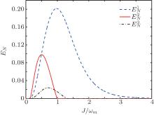
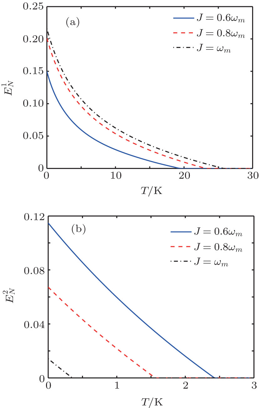
Firstly, we will study the optomechanical entanglement in two coupled cavities case. In order to investigate the behavior of CV entanglement between the elements of the tripartite system in this case, we will denote the logarithmic negativity for the mirror– cavity 1, mirror– cavity 2, and cavity 1– cavity 2 entanglements as , , and respectively. In our numerical calculations, we will use the set of parameters for the optomechanical system given in Table 1, which match the current experimental state, thus making our proposal very close to feasibility.

Table 1.

Table 1.

Table 1. The parameters used in our numerical calculations, taken from the experiments in Ref. [35]. Paramter Symbol Value Mechanical mass m 5 ng Mechanical frequency ω m/2π 100 Hz Mechanical damping rate γ m/2π 100 Hz Cavity length L 1 mm Input power P 50 mW Cavity– field wavelength λ 810 nm Optical damping rate κ 34.1 MHz

Table 1. The parameters used in our numerical calculations, taken from the experiments in Ref. [35].

For the sake of simplicity, we assume . In Fig. 2, we have plotted the three bipartite logarithmic negativities (dashed curves), (solid curves), and (dash– dotted curves), versus the normalized detuning Δ /ω _m at a fixed temperature of T = 400 mK for four values of the coupling strength J = 0.4ω _m (Fig. 2(a)), J = 0.6ω _m (Fig. 2(b)), J = 0.8ω _m (Fig. 2(c)), and J = ω _m (Fig. 2(d)). It can be clearly seen that the bipartite entanglement is enhanced while the bipartite entanglement is decreased and the bipartite entanglement is almost unchanged with the increase of J. That is to say, the entanglement between mirror and cavity 1 (remote cavity) increases at the expense of mirror and cavity 2 (adjacent cavity) entanglement, and the adjacent cavity serves as an entanglement transmitter in this process. More importantly, under the increasing action of cavity– cavity coupling, the range of the entanglement between two distant subsystems (mirror and cavity 1) can be broader, i.e., from Δ /ω _m ∈ [0.5, 1.5] in Fig. 2(a) to Δ /ω _m ∈ [0.3, 2] in Fig. 2(d). The more broader effective detuning is obtained, the more easily it is realized in experiment.

Fig. 2.

	Figure Option ViewDownloadNew Window
	Fig. 2. Plot of the logarithmic negativity (dashed curves), (solid curves) and (dash– dotted curves) as a function of the normalized detuning Δ /ω m at a fixed temperature T = 400 mK. (a) J = 0.4ω m, (b) J = 0.6ω m, (c) J = 0.8ω m, (d) J = ω m.

Fig. 3.

	Figure Option ViewDownloadNew Window
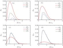
	Fig. 3. Plot of the logarithmic negativity (dashed curves), (solid curves), and (dash– dotted curves) versus the coupling strength J when Δ 1 = − ω m, Δ 2 = ω m.

Fig. 4.

	Figure Option ViewDownloadNew Window
	Fig. 4. Plot of the logarithmic negativities (a) and (b) versus the environment temperature when Δ 1 = − ω m, Δ 2 = ω m. The solid, dashed, and dash– dotted lines are corresponding to different coupling strengths J = 0.6ω m, 0.8ω m, and ω m, respectively.

For clearly presenting the effect of cavity– cavity coupling strength on the optomechanical entanglement, we plot , , and with respect to J in Fig. 3 where cavity 1 is driven on the blue sideband, Δ ₁ = − ω _m, and cavity 2 on the red sideband, Δ ₂ = ω _m. This figure shows that the three bipartite entanglements increase first and go through a peak at about J = ω _m (dashed line), J = 0.5ω _m (solid line), J = 0.75ω _m (dash– dotted line), then drop close to zero. It is worth noting that the optimal entanglement between mirror and cavity 1 is reached at J = ω _m when the entanglement between mirror and cavity 2 disappears completely at this point. In our scheme there is no direct interaction between the cavity 1 and mirror, so one may say that the entanglement is entirely transferred from the adjacent cavity to the distant cavity due to the cavity– cavity coupling. Hence, the optomechanical entanglement between the mechanical mode and the optical mode is very sensitive to the coupling strength J. This result reveals that by changing the value of J, one can control the entanglement distribution in the tripartite system, which implies that we can transfer the entanglement to two indirectly coupled subsystems through the coupling of two cavities.

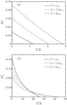
It is also important to understand the behavior of entanglement with respect to the temperature T. We finally discuss the robustness of optomechanical entanglement ( and ) with respect to the environmental temperature, which is shown in Fig. 4. We can see that the optomechanical entanglement between mirror and cavity 1 persists for temperatures above 19 K, as illustrated in Fig. 4(a). Moreover, the logarithmic negativity and its critical value of temperature T_c increase with the increase of J (T_c is defined as T > T_c, E_N = 0). However the entanglement of mirror– field 2 is fragile to the environment temperature which disappears at about 2 K. In addition, the stronger the coupling strength, the smaller the logarithmic negativity , and the lower the critical value of temperature T_c, as seen in Fig. 4(b).

3.2.Numerical calculation for three-cavity case

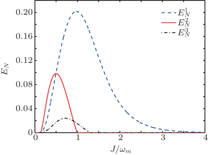
Then we will investigate the optomechanical entanglement properties in the case of three coupled cavities. In this case, we mainly discuss the entanglement between the three cavities and mirror since the entanglement between three cavities is too small. We will denote the logarithmic negativities for the mirror– field 1, mirror– field 2, and mirror– field 3 bimodal partitions as , , , respectively. In the following numerical calculations, the system parameters are taken as the same as the case of two coupled cavities. We also assume for simplicity. The three bipartite logarithmic negativities (dashed curves), (solid curves), and (dash– dotted curves) versus the normalized detuning Δ /ω _m are shown in Fig. 5. It is clearly seen that the optimal entanglement is reached at about Δ /ω _m = 0.5. Moreover, the largest entanglement is the one between the mirror and cavity 2 when J = ω _m, which are indirectly coupled, as seen in Fig. 5(a). With the increasing of coupling strength, the logarithmic negativity decreases, while the logarithmic negativities and increase. We also observed in Fig. 5(d) that the degree of entanglement for mirror– cavity 1 has a similar curve to that of mirror– cavity 3 for a large coupling strength. When J = 5ω _m, the entanglement between mirror and cavity 1 (3) reaches its maximum 0.15 at about Δ = 0.5ω _m. At the same time, the entanglement between mirror and cavity 2 decreases to 0.02. This indicates that the entanglement is transferred from the middle cavity 2 to cavities (1 and 3) on both sides of cavity 2 with the increase of the coupling strength.

Fig. 5.

	Figure Option ViewDownloadNew Window
	Fig. 5. Plot of the logarithmic negativity (dashed curves), (solid curves), and (dash– dotted curves) as a function of the normalized detuning Δ /ω m. (a) J = ω m, (b) J = 1.5ω m, (c) J = 2.5ω m, (d) J = 5ω m.

In Fig. 6, we also plot the logarithmic negativity , , and as a function of the coupling strength J when , Δ ₂ = − ω _m, and T = 400 mK. It is seen obviously from the figure that the maximum entanglement between the mirror and cavity 2 is obtained near J/ω _m = 1, and the logarithmic negativity disappears rapidly with the sufficiently large coupling strength J (solid curve). However, the entanglement between the mirror and cavity 1 (3) is enhanced and becomes more stable with the increase of J, which is quite different from Fig. 4. This implies that we can obtain stationary entanglement between two distant subsystems through adjusting the parameter J.

Fig. 6.

	Figure Option ViewDownloadNew Window
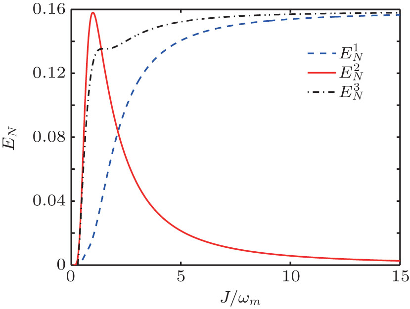
	Fig. 6. Plot of the logarithmic negativity (dashed curve), (solid curve), and (dash– dotted curve) versus the coupling strength J when , Δ 2 = − ω m.

The robustness of the optomechanical entanglement , with respect to temperature T is shown in Figs. 7(a) and 7(b), respectively. From this figure, we can see that the entanglement between mirror and cavity 1 rapidly decreases from 0.09 to zero with the environment temperature from 0.1 mK to 3 K when J = 2ω _m (dash– dotted line in Fig. 7(a)). Furthermore, the logarithmic negativity and its critical value of temperature T_c increase with the value of J. It is worth noticing that the entanglement of mirror– cavity 2 becomes more robust to temperature (T_c = 40 K, as shown in Fig. 7(b)) although the degree of entanglement decreases with the increasing of J.

Fig. 7.

	Figure Option ViewDownloadNew Window
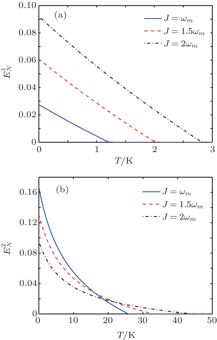
	Fig. 7. Plot of the logarithmic negativity (a) and (b) versus the environment temperature when , Δ 2 = − ω m. Solid, dashed, and dash– dotted curves refer to different coupling strengths J = ω m, 1.5ω m, 2ω m.

In conclusion, we have studied the properties of optomechanical entanglement in a coupled cavity– array with a movable mirror through the logarithmic negativity. We mainly considered two cases of a different number of coupled cavity (two and three cavities). Our results show that the entanglement of the adjacent cavity and mirror can be entirely transferred to the remote cavity and mirror due to cavity– cavity coupling in the case of two coupled cavities. Such an optomechanical entanglement between the distant cavity mode and the mechanical mode of the mirror is sensitive to cavity– cavity coupling strength and cavity– pump detunings. The stationary distant entanglement can be achievable through strong cavity– cavity coupling when , Δ ₂ = − ω _m in the case of three coupled cavities. It is worth noting that the generated remote entanglement is surprisingly robust against increasing temperature: entanglement may persist above 19 K and 25 K in the two cases. According to our theoretical calculations and analyses, we believe that if we continue to increase the number of cavities, the middle cavities can serve as a signal transmission medium to realize quantum information transfer processing from the nearest cavity to the farthest cavity.