
Synchronization of coupled chaotic Hindmarsh Rose neurons: An adaptive approach
[Wei Wei† ]
]
]
|
|


†Corresponding author. E-mail: weiweizdh@126.com
*Project supported by the Beijing Natural Science Foundation, China (Grant No. 4132005), the National Natural Science Foundation of China (Grant No. 61403006), the Importation and Development of High-Caliber Talent Project of Beijing Municipal Institutions, China (Grant No. YETP1449), and the Project of Scientific and Technological Innovation Platform, China (Grant No. PXM2015_014213_000063).
In this paper, we consider the synchronization of chaotic Hindmarsh Rose (HR) neurons via a scalar control input. Chaotic HR neurons coupled with a gap junction are taken into consideration, and an active compensation mechanism-based adaptive control is employed to realize the synchronization of two HR neurons. As such an adaptive control is utilized, an accurate model of the system is of no necessity. Asymptotical synchronization of two HR neurons is guaranteed by theoretical results. Numerical results are also provided to confirm the proposed synchronization approach.
Chaos is a very important phenomenon in nonlinear science. Synchronization of chaotic systems attracts a great deal of interest and attention from science and engineering fields, owing to its potential applications in various scientific disciplines, such as physics, chemistry, biology, secure communication, and other areas.[1– 3] Particularly, the synchronization of coupled neurons has been suggested as an important mechanism for accomplishing critical functional goals including biological information processing in the brain, [4, 5] and the production of regular rhythmical activity.[6] The presence, absence, and the degree of synchronization can be crucial factors of function or dysfunction for a biological system.[7] Therefore, the synchronization of neural systems has been extensively studied.
With an attempt to understand the dynamics of neurons and the synchronization phenomena of biological neural networks, various neuron models have been proposed. The first complete mathematical model describing neural membrane dynamics, i.e., the Hodgkin– Huxley (HH) model, was proposed by Hodgkin and Huxley in 1952.[8] Since then, other neuronal models have also been published, such as the FitzHugh– Nagumo (FHN) model, [9] the Hindmarsh– Rose (HR) model, [10] the Chay model, [11] the Morris– Lecar model, [12] the Leech model, [13] and the Ghostburster model.[14] The synchronization mechanism between neurons can be classified as two classes. One depends on natural coupling, in which the synapse types and internal noises are key factors in synchronization, and the other depends on the artificial coupling, in which an explicit control signal is applied in order to achieve synchronization. For the natural coupling, it can be found in biophysical experiments and neural systems have been modeled based on experimental results. Both biophysical experimental results and theoretical analysis of neural systems have confirmed that natural coupling does produce synchronization among neurons.[15– 17] For the second synchronization mechanism, a variety of synchronization approaches have been proposed to synchronize the aforementioned neural systems.[18– 26] In Ref. [18], H∞ variable universe adaptive fuzzy control is utilized to synchronize the HH neurons. Adaptive neural network H∞ control, [19] state observer based control, [20, 21] nonlinear feedback control, [22– 24] robust adaptive sliding mode control, [25] and adaptive control[26] have been utilized to realize the synchronization of various neural systems. In addition, a novel master-slave coupling, which exists between the membrane potential of the master neuron and the slow ion kinetics of the slave neuron, other than classical synchronization of two neurons modeled as electrical and chemical coupling in action potential variables, enables the synchronization between neurons.[27] Such a connection can also be viewed as an artificial coupling, since, from the neuroscience and molecular biology point of view, such a connectivity between neurons is hard to explain. Based on the novel coupling, exponentially fast synchronization between two HR neurons has been reported in Ref. [27]. Recently, a network of HR neurons was built and analyzed.[28] Most of the aforementioned methods and many other reported synchronization approaches, to a great extent, focus on the synchronization of two neurons with faithful models. However, uncertainties are ubiquitous, and a synchronization approach which is independent of the faithful model of neural systems is in great need both from a theoretical and a practical point of view. Additionally, in order to achieve the synchronization, some methods are developed based on the full control inputs for all of the system states, i.e., each state has one control signal.[19, 22] Actually, some states of a neuron model are not able to obtain signals from an external electric field, and it is not practical to realize those approaches. Two identical HR neuronal chaotic systems are synchronized by a state observer-based control.[20] An adaptive control approach[26] is proposed to synchronize two HR neurons with unknown parameters. However, no disturbance is considered in those synchronizations. In fact, disturbance is very common in applications. It is practical to consider the disturbance in the design of control. Therefore, the synchronization approach using a scalar control input, which is robust enough to uncertainties and disturbance, is in great need in practice.
In this paper, an adaptive controller based on an active compensation mechanism is adopted to synchronize two HR neurons under different external stimulations. All of the unknown nonlinear functions, uncertainties, and disturbance can be observed and actively compensated for by the disturbance observer existing in the adaptive controller, and the synchronization of two coupled HR neurons is achieved. The proposed synchronization method is confirmed by both theoretical and numerical results.
The rest of this paper is organized as follows. In Section 2, the HR neuron model is given. The synchronization of two coupled HR neurons is formulated and an adaptive controller based on an active compensation mechanism is designed to synchronize two coupled HR neurons in Section 3. Simulation results are given in Section 4 to confirm that the controller is capable of realizing the synchronization of two coupled HR neurons. Finally, conclusions are drawn in Section 5.
The model of an HR neuron is described by a group of three-dimensional nonlinear differential equations:[25]
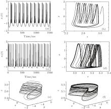
where x is the membrane potential, y is a recovery variable associated with the fast current of Na+ or K+ ions, and z is the adaptation current associated with the slow current of Ca2+ ion. Here, a = 1, b = 3, c = 1, d = 5, s = 4, r = 0.006, x0 = − 1.6, and Iext is the external current input. For different values of Iext, the dynamics of membrane potential x varies (see Fig. 1). When Iext = 3.2, the dynamic behavior of the membrane potential is chaotic, and when Iext = 2.8, the dynamic behavior of the membrane potential is periodic. The waveforms of membrane potentials and phase portraits (on the x– z plane and x– y– z plane) are helpful to distinguish the two qualitatively different behaviors.
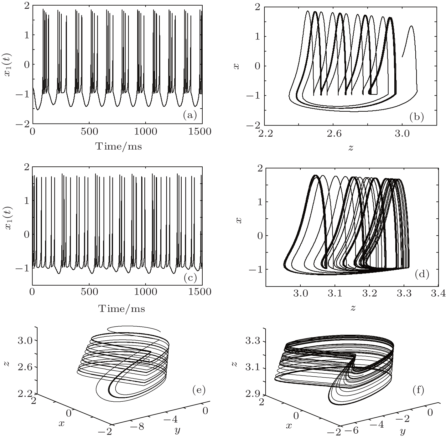 | Fig. 1. Dynamic behaviors of an HR neuron, showing [(a) and (c)] membrane potentials when Iext = 2.8 (periodic) and Iext = 3.2 (chaotic), [(b) and (e)] phase portraits in the planes x– z and x– y– z when Iext = 2.8 (periodic), and [(d) and (f)] phase portraits in the planes x– z and x– y– z when Iext = 3.2 (chaotic). |
In this section, the adaptive synchronization of two HR neurons coupled with a gap junction will be considered. The master and slave neurons are given below.
The master neuron:
and the slave neuron:
where a, b, and c are assumed to be unknown; g is the coupling coefficient, which is also assumed to be unknown; Imext and Isext are external current inputs applied to the master neuron and slave neuron respectively; u is a scalar control signal utilized to synchronize two coupled HR neurons. In this paper, we define synchronization errors as

then the error dynamical system can be derived by subtracting master neuron (2) from slave neuron (3), i.e.,
where

Our work is to design controller u, which drives the states of the slave neural system to track those of the master neural system, i.e., to realize 

if nonlinear function f (• ) is exactly known.
Here h0 > 0 is the feedback gain, then error dynamical system (4) can be rewritten as

By choosing a proper value of h0, error variable e1 converges to zero, and then the zero dynamics of error dynamical system (4) will also be stable.[29] Therefore, the ideal control law u* is able to drive the trajectories of the synchronization error dynamical system to be zero asymptotically.
However, nonlinear function f (• ), in general, is always unknown. Thus, the ideal controller u* is not feasible in practice.
Comparing with identifying nonlinear function f (• ), we may see that estimation and compensation of f (• ) are more practical. This is the main idea of most disturbance observer-based control approaches. According to such an idea, in this paper, an adaptive control is also employed. The controller employed is able to estimate and compensate for f (• ) in real time, which will guarantee the nice performance of synchronization.
The active compensation-based adaptive controller can be written as
where zi, i = 1, … , n are system states; parameters hi, ki, i = 0, 1, … , n − 1 are tunable parameters, hi are chosen so that eigenvalues of polynomial h(s) = sn + hn − 1sn− 1 + · · · + h1s + h0 are in the open left half-plane; 
In fact, uncertainties are ubiquitous. It is significant that nice performance will still hold even if uncertainties exist. The disturbance observer
The control law, when the relative degree is one, is shown as follows:
where
Control law (8) utilized in this paper will estimate and compensate for the nonlinear function and disturbance by disturbance observer
Theorem 1 There exists a constant μ * > 0, such that if k0 > μ * , then closed-loop error dynamical system (14) is asymptotically stable.
Proof For error dynamical system (4), the active compensation control law u can be represented as

Substituting Eq. (9) into error dynamical system (4), we have

where 


The derivatives of d and


then

Therefore the closed-loop system is

Supposing that V is a differentiable positive-definite function of e1, i.e.,

Then the compact domain

can be defined. M is an arbitrary positive constant. Thus, for any h0 > 0 and any e1 ∈ UV, M, there are

Stabilize closed-loop system (14), then a Lyapunov function candidate will be defined as

For a fixed M, let UW, M be a compact domain such that

Differentiating W along system (14), we have

It is obvious that the projection of UW, M onto the hyperplane d̃ = 0 coincides with UV, M. Thus expressions 1) and 2) also hold for ∀ (e, d̃ ) ∈ UW, M. According to Ref. [30], we have the following technical lemmas

then


where PV and Pα are positive and dependent on M. Therefore, for any ∀ (e, d̃ ) ∈ UW, M, we have

According to the Sylvester criterion, it is straightforward to obtain the following inequality:

Let

thus, if k0 > μ * , Ẇ is negative-definite in UW, M, and closed-loop system (14) is asymptotically stable in UW, M.
The closed-loop error dynamical system is asymptotically stable, which means that the synchronization between master and slave neural systems is achieved.
In this section, the numerical simulations are presented to verify the active compensation-based adaptive controller utilized in the present paper. The initial states are chosen as follows: [xm(0), ym(0), zm(0)]T = [0.3, 0.3, 3.0]T and [xs(0), ys(0), zs(0)]T = [0.1, 0.6, 2.0]T, respectively. Coupling coefficient g is selected to be 0.2. In the following simulations, the simulation time is 4000 ms, and control actions will be activated at 1600 ms. The parameters of adaptive controller u are chosen to be k0 = h0 = 20. Three cases are considered.
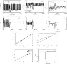
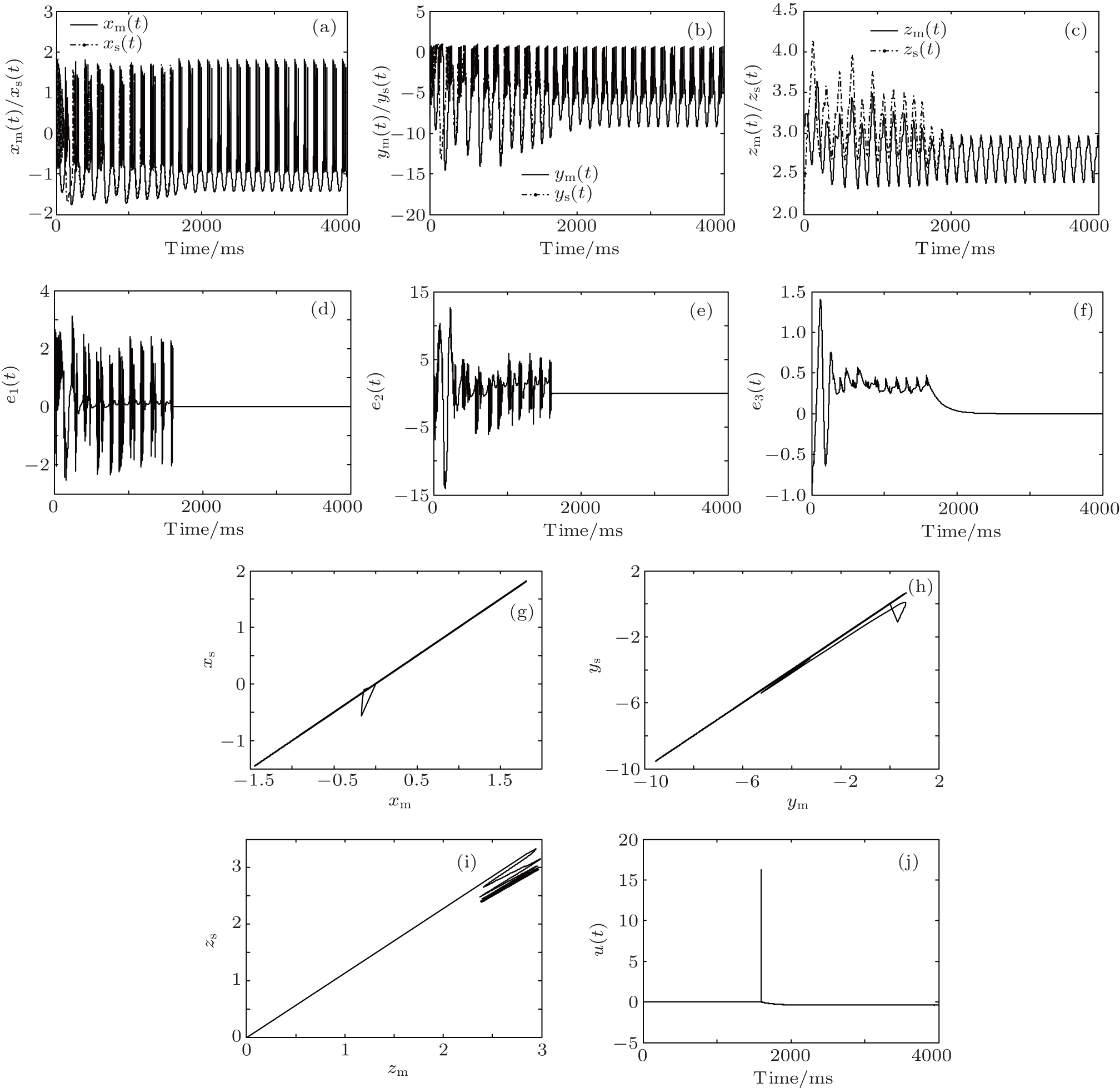
Case 1 External stimulus of the master neuron is chosen to be 3.2, and the stimulus of the slave neuron is 2.8. We aim to drive the slave neuron system, which exhibits periodic behaviors, to track chaotic behaviors of the master neuron system. The time traces of system states, synchronization errors, phase plane diagram after control action has been applied, and control input are shown in Fig. 2.
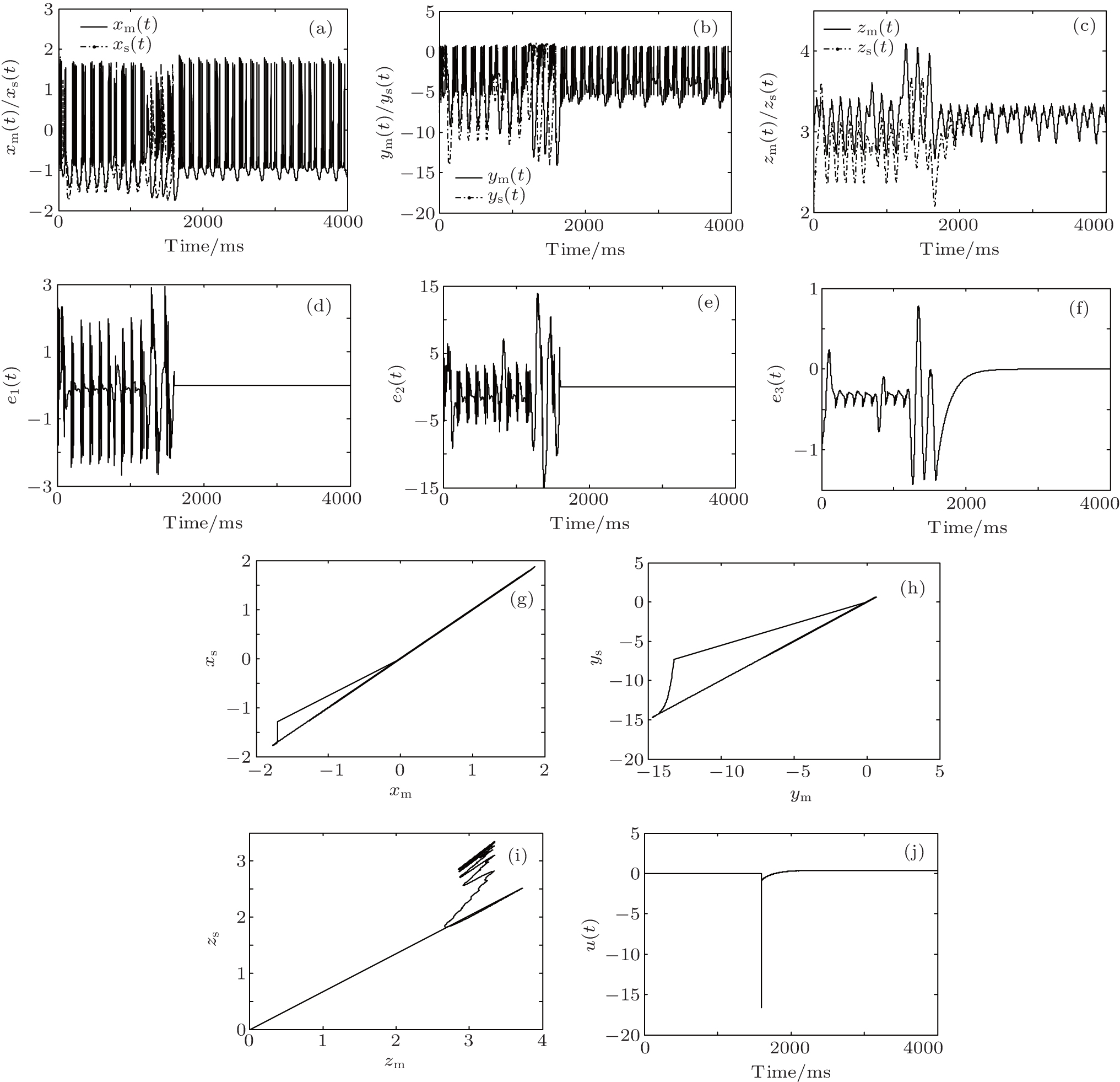 | Fig. 2. Synchronizations between two HR neurons via active compensation control (periodic behavior tracks chaotic behavior), showing (a) time traces of system states xm and xs, (b) time traces of system states ym and ys, (c) time traces of system states zm and zs, (d) synchronization errors between xm and xs, (e) synchronization errors between ym and ys, (f) synchronization errors between zm and zs, (g) phase plane diagram of xm and xs after control action has been activated, (h) phase plane diagram of ym and ys after control action has been activated, (i) phase plane diagram of zm and zs after control action has been activated, and (j) control signal for synchronization. |
Case 2 External stimulus of the master neuron is chosen to be 2.8, and the stimulus of the slave neuron is 3.2. We aim to drive the slave neuron system, which exhibits chaotic behaviors, to track periodic behaviors of the master neuron system. The time traces of system states, synchronization errors, phase plane diagram after the control action has been applied, and control input are shown in Fig. 3.
 | Fig. 3. Synchronizations between two HR neurons via active compensation control (chaotic behavior tracks periodic behavior), showing (a) time traces of system states xm and xs, (b) time traces of system states ym and ys, (c) time traces of system states zm and zs, (d) synchronization errors between xm and xs, (e) synchronization errors between ym and ys, (f) synchronization errors between zm and zs, (g) phase plane diagram of xm and xs after control action has been activated, (h) phase plane diagram of ym and ys after control action has been activated, (i) phase plane diagram of zm and zs after control action has been activated, and (j) control signal for synchronization. |
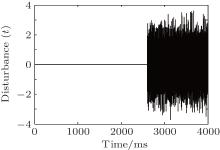
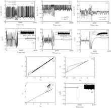
Case 3 Under the same condition as Case 1, and a disturbance signal is added at 2600 ms. The disturbance signal is random noise, and its intensity is 0.1. It is shown in Fig. 4. We aim to drive the slave neuron system, which exhibits periodic behaviors, to track chaotic behaviors of the master neuron system, when the disturbance exists. The time traces of system states, synchronization errors, phase plane diagram after control action has been applied, and control input are shown in Fig. 5.
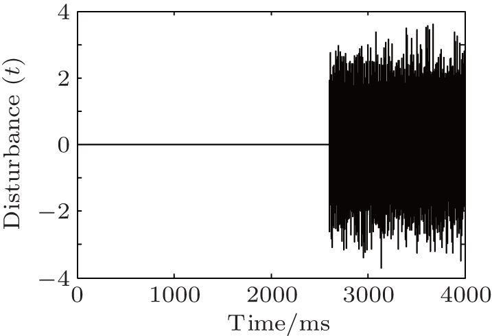 | Fig. 4. Disturbance signal. |
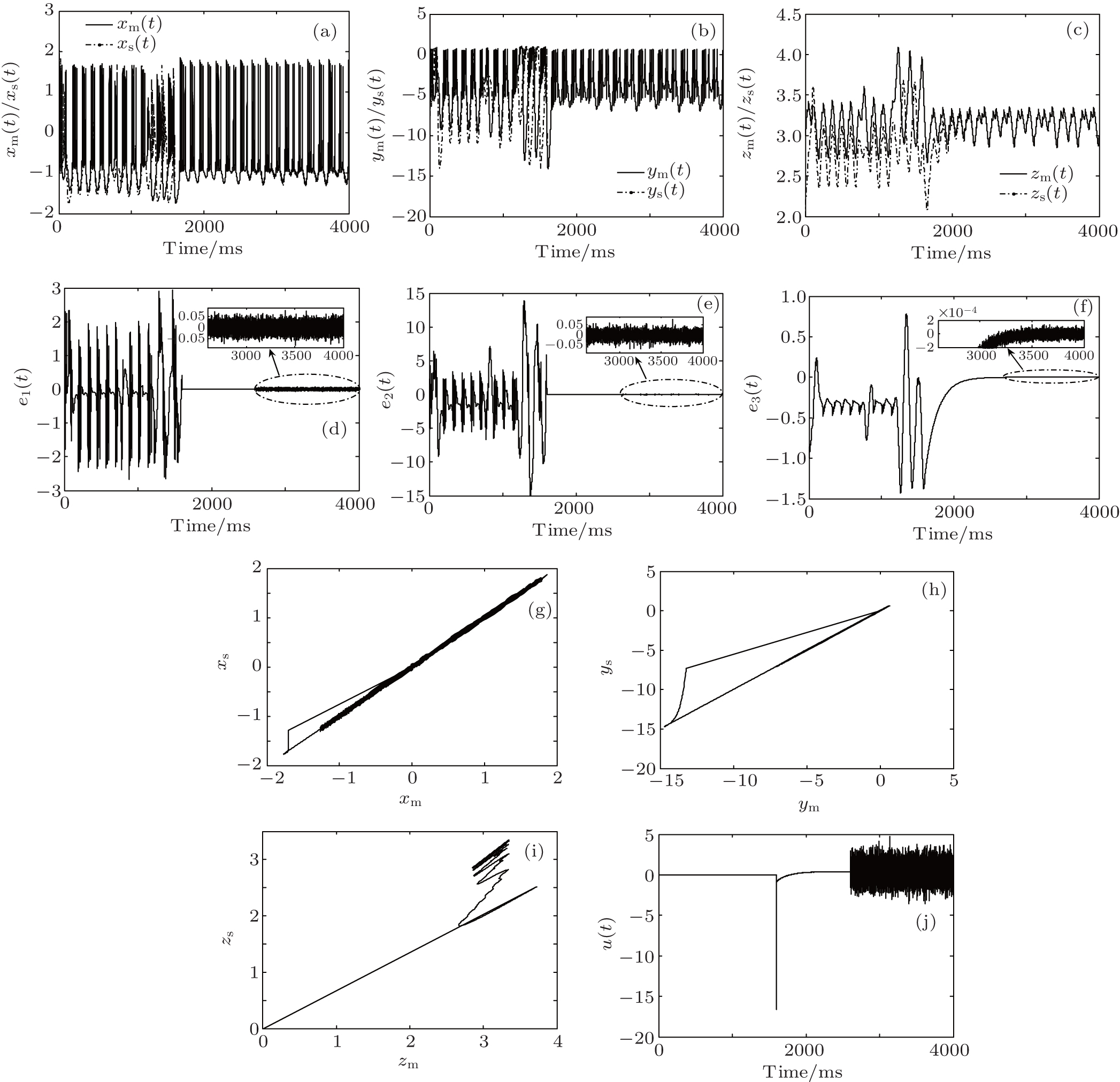 | Fig. 5. Synchronizations between two HR neurons via active compensation control (disturbance exists), showing (a) time traces of system states xm and xs, (b) time traces of system states ym and ys, (c) time traces of system states zm and zs, (d) synchronization errors between xm and xs, (e) synchronization errors between ym and ys, (f) synchronization errors between zm and zs, (g) phase plane diagram of xm and xs after control action has been activated, (h) phase plane diagram of ym and ys after control action has been activated, (i) phase plane diagram of zm and zs after control action has been activated, and (j) control signal for synchronization. |
From the simulation results of Cases 1– 3, we can see clearly that the active compensation-based adaptive control can realize the synchronization between two coupled HR neurons successfully, even if the disturbance exists.
In this paper, the synchronization between two coupled HR neurons is investigated. The theoretical and simulation results both show that the active compensation-based adaptive control can achieve the synchronization of HR neurons effectively. Perfect knowledge of the neural systems is not required. By choosing proper controller parameters, the synchronization can be realized. This is of great importance in practice, because uncertainties are ubiquitous, it is not practical to develop exact models.
It is worth pointing out that although the synchronization of coupled HR neurons is considered in this paper, the adaptive control adopted only needs the membrane potential information of the neuron, i.e., little amount of neuronal information is needed, which indicates that it can be generalized to the synchronization of other neural systems, or even in the synchronization of biological neural networks, which is the work we are doing now.
| 1 |
|
| 2 |
|
| 3 |
|
| 4 |
|
| 5 |
|
| 6 |
|
| 7 |
|
| 8 |
|
| 9 |
|
| 10 |
|
| 11 |
|
| 12 |
|
| 13 |
|
| 14 |
|
| 15 |
|
| 16 |
|
| 17 |
|
| 18 |
|
| 19 |
|
| 20 |
|
| 21 |
|
| 22 |
|
| 23 |
|
| 24 |
|
| 25 |
|
| 26 |
|
| 27 |
|
| 28 |
|
| 29 |
|
| 30 |
|