A novel adaptive-impulsive synchronization of fractional-order chaotic systems
[Andrew Leung Y. T.†a)  , Xian-Feng Li
a) , Yan-Dong Chub) , Hui Zhangc) ]
, Xian-Feng Li|
|


†Corresponding author. E-mail: aytleung@gmail.com
*Project supported by the National Natural Science Foundations of China (Grant Nos. 11161027 and 11262009), the Key Natural Science Foundation of Gansu Province, China (Grant No. 1104WCGA195), the Specialized Research Fund for the Doctoral Program of Higher Education of China (Grant No. 20136204110001).
A novel adaptive–impulsive scheme is proposed for synchronizing fractional-order chaotic systems without the necessity of knowing the attractors’ bounds in priori. The nonlinear functions in these systems are supposed to satisfy local Lipschitz conditions but which are estimated with adaptive laws. The novelty is that the combination of adaptive control and impulsive control offers a control strategy gathering the advantages of both. In order to guarantee the convergence is no less than an expected exponential rate, a combined feedback strength design is created such that the symmetric axis can shift freely according to the updated transient feedback strength. All of the unknown Lipschitz constants are also updated exponentially in the meantime of achieving synchronization. Two different fractional-order chaotic systems are employed to demonstrate the effectiveness of the novel adaptive–impulsive control scheme.
Fractional calculus can describe physical phenomena and mathematical models more accurately than the classical integer calculus[1– 3] and has many applications in interdisciplinary fields.[4– 9] The applications of fractional calculus to physics, [5] engineering, [6] signal processing, [7] and control processing[8] have attracted a great deal of attention recently. In comparison with traditional integer-order control, the fractional-order control is more general and becoming more popular because of its flexibility and integrity.[9] Intensive studies confirmed theoretically and physically that the chaotic and hyperchaotic behaviors exist the nonlinear fractional-order systems.[3, 8– 15] Meanwhile, synchronization of fractional-order chaotic systems also has attracted increasing attention due to its potential applications in secure communication[16, 17] and digital cryptography.[18– 20] A variety of control schemes have been proposed to control and synchronize fractional-order chaos in infinite or finite time, [21, 22] such as active control, [23, 24] sliding mode control, [25– 27] adaptive control, [28] passive control, [29] and impulsive control.[30– 34] Both fractional-order models and controllers have more degrees of freedom besides memory and hereditary effects.[8] A consensus is arising that chaotic synchronization of fractional-order systems has more advantages and real objects than that of integer order systems.
Impulsive control is a control paradigm based on impulsive differential equations and has been applied in some areas with inherited impulsive properties, such as neurobiology and genetics, economics, and ecology. In realizations, the control actions are imposed on a control plant at certain discrete instants. It has been found that it is important on synchronizing complex systems via impulsive control, [31– 43] and is more suitable for digital implementation of secure communication in comparison with other schemes.[41] Since the impulsive control allows the stabilization of the controlled plant using only small impulsive actions, the overall control cost would be reduced. Therefore, it is more suitable for dealing with the systems that cannot endure continuous strong disturbance.[35] Heretofore, most impulsive controllers are designed in the framework of Lyapunov asymptotic stability based on the comparisons method developed in Ref. [41]. Different restriction relations are necessary due to different designs and repetitive calculations. For example, one has to compute the maximum eigenvalues of some matrices and then examine whether they meet some assigned inequalities. In this case, previous works would rather check these restriction relations many times and estimate the error vectors of states than utilize the comparison method directly. Furthermore, in order to seek the control gains, the nonlinear functions in the drive system and response system should be immersed in some rigorous mathematical constraints. The estimations of Lipschitz conditions of nonlinear functions and their bounded norms in Euclidean space are two common conditions. However, it is very hard to work out the local Lipschitz constant for every nonlinear equation in practice. In addition, the initial difference between two systems is huge but the final controlled errors cannot be constant although small. The bounded norms of them are always evaluated with the boundaries of orbits in the phase space. As a result, these loose approaches always trigger improper outcomes. For instance, the coupling strengths may be very big or unequal, which in experience may bring out unexpected dynamical behavior, such as desynchronization bursts. Such a desynchronization burst is usually overlooked or difficult to be found because it always starts after a long synchronization moment. The combination of adaptive and impulsive controls partly makes up for the aforementioned imperfections and is easy to achieve synchronization. Alternatively, the variable feedback strength can be automatically adapted to completely synchronize two chaotic systems. In an augment system, the adaption terms are linearly relying on the errors in variables but vanish once the synchronization is achieved. Although this combination scheme is very analytical and has been extended extensively, [33, 44– 49] the feedback strength is never considered to be updated with an adaptive law. This is because both the transient and the final feedback strengths at every impulsive constant are not sure of falling into the admissible region. Furthermore as far as we know, the adaptive– impulsive synchronization on fractional-order chaotic systems is rarely considered to this day.
In this paper, a novel adaptive– impulse synchronization scheme is proposed to achieve synchronization of fractional-order chaotic systems. The nonlinear equations in the chaotic systems considered here suffer unknown local Lipschitz constants. In order to guarantee the convergence is no less than an expected exponential rate, a combined feedback strength design is created. At the impulsive instants, rational constant feedback strengths neutralize the updated transient and the ultimate feedback strengths such that the symmetric axes can shift freely. Whereby, the combined feedback strength at every impulsive instant is surely falling in the admissible region. Both impulse intervals and the feedback strength are derived from one criterion that is also associated with unknown local Lipschitz constants, and the rate of convergence we expected. The criterion is completely adaptive to implement in locating the admissible region of control strengths to ensure the occurrence of synchronization. All of the unknown local Lipschitz constants will be identified dynamically with adaptive laws in the process of achieving synchronization, rather than estimated from the attractors bounds in the initial state. Finally, an autonomous hyperchaotic system and a non-autonomous fractional-order chaotic system are employed to demonstrate the effectiveness and the feasibility of the proposed scheme.
The fractional-order integro-differential operator is the extending concept of integer order integro-differential operator. It can be described by a fundamental operator as follows:
where α is the fractional order, which can be complex. The constants a and t are the limits of the operation. There are many ways to define fractional-order integral and derivative.[1] Two definitions are generally used, namely Riemann– Liouville and Caputo definitions. In considering functions with initial conditions, the Caputo fractional derivative will be used through the paper.
The Caputo derivative of order α is given as[1]

where, m = ⌈ α ⌉ is a least integer no less than α . The fractional-order α here is limited as 0 < α ≤ 1. Γ (· ) denotes the Euler’ s Gamma function. For the sake of convenience in writing, the Caputo fractional-order fundamental operator 
Recently, many numerical methods have been proposed for simulating the fractional-order systems. Amongst these methods, some reliable ones that were proposed in Refs. [50]– [54] are all very effective. Through this paper, a Jacobian predictor– corrector algorithm is employed to simulate the numerical examples. The details and the specific steps of such a scheme can be seen in the appendix of Ref. [52].
Consider a fractional-order chaotic system with initial conditions,
where, k = 0, 1, … , m − 1. x(t) ∈ ℝ n, n ∈ ℕ is the state vector of the system. Assume that the nonlinear function f(t, x(t)) is bounded in the phase space Ω , Ω ⊆ ℝ n × ℝ + . f(t, x(t)): ℝ n × ℝ + → ℝ n is supposed to be 

Remark 1 All the chaotic systems (both in integer order and their fractional-order corresponding parts) can be represented in the form of system (3), such as Chua circuits, Lorenz system, Chen system, Lü system, the unified system and Duffing oscillators.[26] It is hard to work out the accurate Lipschitz constant for every function in a nonlinear system although its attractors are bounded in Ω . Previous researches evaluated the local Lipschitz constants in Ω , which is also an imprecise evaluation from the boundaries of attractors. As stated before, such an evaluation in the initial state is so loose that it is unfit for a dynamical process. To avoid such an imperfection, we assume that all the local Lipschitz constants are unknown a priori. The unknown Lipschitz constants λ ̃ i(t), i = 1, 2, … , n, would be identified dynamically in the course of synchronization, limt→ ∞ λ ̃ i(t) = λ i, i = 1, 2, … , n, and 
In order to achieve synchronization, system (3) is taken as the drive system, while the impulsive-controlled response system is represented as follows,


where y(t) ∈ ℝ n, n ∈ ℕ is the state vector of the response system. The time sequence {tı } of impulsive instants is set as 0 ≤ t0 < t1 < … < tı < … , and tı → ∞ as ı → ∞ . The impulse interval here is not equidistant, 


Define the error state as e(t) = y(t) − x(t). Subtracting system (3) from system (4), we obtain the error dynamical system between them as follows:


The task is to design an adaptive– impulsive controller to achieve the asymptotic synchronization of the drive system (3) and the response system (4), that is, limt→ ∞ ‖ e(t)‖ = 0. As a result, U(ı ) = Δ e(tı ) in (4) is the sole controller at 

where the feedback strength k(t) + k̃ is presented in a combined form, and k̃ is a positive constant concomitant of k(t), which is affirmed that ❘ k(t)❘ > k̃ . More details on k̃ will be given below. The feedback strength k(t) is negative and follows an adaptive law, which is described as

where γ ∈ {0}∪ ℝ + and γ is only configured with an appropriate positive constant at 

However, to the best of our knowledge, there is no efficient scheme to deal with the stability of the fractional-order impulsive differential equation (5a).[32, 33] In order to settle such a problem, equation (4a) will be converted to a corresponding integer-order one by introducing a new function, μ (x(t)) = ẋ (t) − Dα x(t) [33]. Both x(t) and Dα x(t) can be taken from the simulation of system (3). As a result, systems (4) and (5) become


and,


Theorem 1 Suppose that the adaptive feedback strength kı (t) is bounded with the lower bound − e− ρ /2 − k̃ ı − 1 and the upper bound e− ρ /2 − k̃ ı − 1, where − ρ (ρ > 0) is the least convergence exponential rate we expected. Meanwhile, the adaptive law for estimating the Lipschitz constant λ ̃ i is given as

where η i ∈ ℝ + . The error state e(t) in Eq. (9a) will be exponentially stable at a rate no less than e− ρ if the adaptive controller (6) is actuated at 
Proof The candidate Lyapunov function is
Clearly, λ ̃ i(t) is an increasing function such that one has λ ̃ i(tı − 1) ≤ λ ̃ i(t) ≤ λ ̃ i(tı ). In the impulsive interval t ∈ (tı − 1, tı ], the combined feedback strength kı (t) + k̃ ı only is adapted at 
Therefore in the interval of t ∈ (tı − 1, tı ], ı = 1, 2, … , it is represented as

Due to the instant control action (6) at 
From expressions (10) and (12), we can deduce the following formulae. When ı = 1,
Next, when ı = 2,
By repeating the same method, the generalized form is,
where ı = 1, 2, … .
To guarantee the convergence is exponential, we let

As a consequence,

It can be concluded here that 
Recalling expression (13), we have

as t → ∞ .
As shown in expression (19), the convergence rate of error dynamical system (9a) is no less than e− ρ ı . For any given 

The impulsive interval in inequality (21) can be as large as possible, but kı (t) approaches to − (k̃ ı + 1) in the meantime. However, such an ideal strength, kı (t) = − (k̃ ı + 1) in the axis of symmetry, should be avoided because the actual control only activates at the impulsive constants tı , ı = 1, 2, … . In this case, the most rational interval for the combined feedback kı (t) + k̃ ı is
with assuming that tı − tı − 1 ≪ ∞ .
On the other hand, the impulsive interval is determined by the adapted control strength and the identified Lyapunov constant cooperatively at the current impulsive instant. The relationship between them is described as
The impulsive interval τ ı is positive, which implies that

Hereby, the infimum and the supremum of kı (t) + k̃ ı are − 2 and 0 respectively. In the process of synchronization, the adaptive law for feedback strength kı (t) will be updated to a new integration

at an impulsive action. Whereby the concomitant constant k̃ ı can be configured with a positive number in a band depicted in inequality (24), whilst it satisfies kı (t) + k̃ ı ≠ − 1, and so on. Unifying it with the integration of Eq. (10) and the convergence rate we expected, the next impulsive interval τ ı is determined. That is to say the next impulsive instant is fixed. Obviously, the impulsive actions terminate if τ ı < h, where h is the time-step we used for the simulations in the impulsive intervals.
Remark 2 It should be noted here that the axis of symmetry is not controlled by any unpredictable coefficients. It can shift freely to any positive constants according to the transient and ultimate adaptive feedback strengths. One important thing is that regardless of transient time, the costs on the synchronization of two identical chaotic systems are very low. This is an important reason why we confined the combined feedback strength kı (t) + k̃ ı in the admissible region (− 2, − 1) ∪ (− 1, 0) randomly although the endpoints cannot present at any moment. With an expected convergence at exponential rate ρ , the choice on the coefficient in the adaptive law (7) plays an important role because it determines the estimation of kı (t), while guaranteeing the impulsive interval 0 < τ ı ≪ ∞ . Such an almost insolvable problem has to be handled by a posteriori means.[55]
The first example is a four-dimensional (4D) novel fractional-order hyperchaotic system. The equations of the system are described as[56, 57]

where, μ , ν , a, b, c, and d are positive parameters.
Like its integer-order version, [58] system (25) has only one equilibrium E0 = {0, 0, 0, 0}. As it has been proved, [58] system (25) has a unique solution for some time tℓ , ℓ ∈ ℝ + . It also can be hyperchaotic because it has two positive Lyapunov exponents if the fractional order α = 0.97 and the parameters μ = 35, ν = 100, a = 35, b = 4, c = 25, and d = 5, respectively.
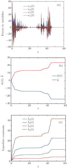
When the time-step h = 10− 3, the coefficients γ = 0.1 and η i = 0.1, i = 1, 2, 3, 4, the numerical results are depicted in Figs. 1(a)– 1(c). In these simulations, the combined feedback strength is uniform, i.e., k̃ ı = − kı (tı ) − 0.5 at every impulse instant. The exponential convergence rate we expected is not less than ρ = 1. The initial conditions for the drive system and the response system are x0 = {0.1}4 and y0 = {10.1}4, respectively. To make sure that the adaptive control strength (7) is always negative, the initial condition for Eq. (7) is a negative random number. For a similar reason, the initial conditions for Eq. (10) are four positive random numbers.
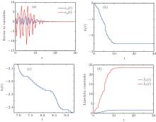
The fractional-order Duffing system is taken as the second example to illustrate the effectiveness of the proposed novelty synchronization scheme. The existence and uniqueness about the fractional-order Duffing system were well studied.[24] The equations of the system are described as
where, a, b, c, and f are the parameters, and ω is the frequency of the force term. With commensurate fractional order α = 0.98, it is chaotic when the parameters are specified as a = b = 1, c = 0.2, and f = 25.5, ω = 1. The initial condition for the drive is x0 = (0.9, 0.01), while the initial condition for the response systems is y0 = (2, 3). With same configurations as example 1 for the time-step h, the coefficients γ , and η i, i = 1, 2 the numerical results are depicted in Figs. 2(a)– 2(d). In these simulations, the combined feedback strength is random, i.e., k̃ ı = − kı (tı ) + ℜ , ℜ ∈ (− 2, − 1) ∪ (− 1, 0) at every impulse instant. The initial settings for the remnants of the argument system are the same as example 1.
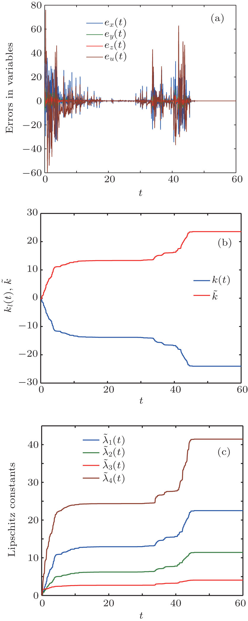 | Fig. 1. Numerical simulations of example 1. (a) Errors in variables, (b) the estimations of kı (t), and (c) the evaluations of Lipschitz constants. |
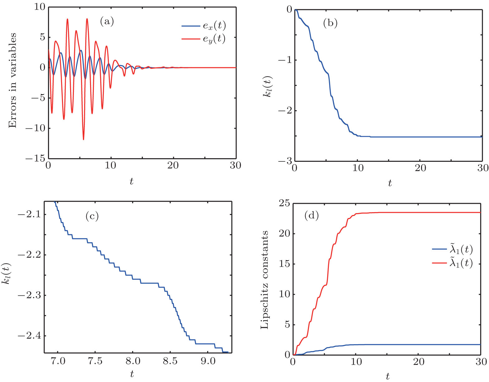 | Fig. 2. Numerical simulations of example 2. (a) Errors in variables, (b) the estimations of kı (t), (c) the local magnification of Fig. 2(b), and (d) the evaluations of Lipschitz constants. |
In this paper, a novel adaptive– impulsive scheme is proposed for synchronizing fractional-order chaotic systems. The nonlinear functions considered here are supposed to satisfy the local Lipschitz conditions without needing to be known a priori. The combination of adaptive control and impulsive control offers a control strategy gathering the advantages of both. The combined feedback strength design is created to shift the symmetric axis freely according to the updated transient feedback strength. The synchronization converges at an expected exponential rate. All of the unknown Lipschitz constants are also updated to their rational values once the synchronization occurs.
| 1 |
|
| 2 |
|
| 3 |
|
| 4 |
|
| 5 |
|
| 6 |
|
| 7 |
|
| 8 |
|
| 9 |
|
| 10 |
|
| 11 |
|
| 12 |
|
| 13 |
|
| 14 |
|
| 15 |
|
| 16 |
|
| 17 |
|
| 18 |
|
| 19 |
|
| 20 |
|
| 21 |
|
| 22 |
|
| 23 |
|
| 24 |
|
| 25 |
|
| 26 |
|
| 27 |
|
| 28 |
|
| 29 |
|
| 30 |
|
| 31 |
|
| 32 |
|
| 33 |
|
| 34 |
|
| 35 |
|
| 36 |
|
| 37 |
|
| 38 |
|
| 39 |
|
| 40 |
|
| 41 |
|
| 42 |
|
| 43 |
|
| 44 |
|
| 45 |
|
| 46 |
|
| 47 |
|
| 48 |
|
| 49 |
|
| 50 |
|
| 51 |
|
| 52 |
|
| 53 |
|
| 54 |
|
| 55 |
|
| 56 |
|
| 57 |
|
| 58 |
|