
A perturbation method to the tent map based on Lyapunov exponent and its application
[Cao Lv-Chena) , Luo Yu-Ling†a)  , Qiu Sen-Hui
a) , Liu Jun-Xiub) ]
, Qiu Sen-Hui|
|


†Corresponding author. E-mail: yuling0616@gxnu.edu.cn
*Project supported by the Guangxi Provincial Natural Science Foundation, China (Grant No. 2014GXNSFBA118271), the Research Project of Guangxi University, China (Grant No. ZD2014022), the Fund from Guangxi Provincial Key Laboratory of Multi-source Information Mining & Security, China (Grant No. MIMS14-04), the Fund from the Guangxi Provincial Key Laboratory of Wireless Wideband Communication & Signal Processing, China (Grant No. GXKL0614205), the Education Development Foundation and the Doctoral Research Foundation of Guangxi Normal University, the State Scholarship Fund of China Scholarship Council (Grant No. [2014]3012), and the Innovation Project of Guangxi Graduate Education, China (Grant No. YCSZ2015102).
Perturbation imposed on a chaos system is an effective way to maintain its chaotic features. A novel parameter perturbation method for the tent map based on the Lyapunov exponent is proposed in this paper. The pseudo-random sequence generated by the tent map is sent to another chaos function — the Chebyshev map for the post processing. If the output value of the Chebyshev map falls into a certain range, it will be sent back to replace the parameter of the tent map. As a result, the parameter of the tent map keeps changing dynamically. The statistical analysis and experimental results prove that the disturbed tent map has a highly random distribution and achieves good cryptographic properties of a pseudo-random sequence. As a result, it weakens the phenomenon of strong correlation caused by the finite precision and effectively compensates for the digital chaos system dynamics degradation.
Chaos has aroused a research interest in various fields of cryptography due to its inherent random-like behaviours. In the last 20 years, a large number of cryptographic algorithms based on chaos have been proposed[1– 3] and digital chaos systems have been employed in most of these cryptosystems. However, when chaos is realized in computers or digital circuits, a chaos system often suffers dynamical degradation, which refers to the short cycle length, non-ergodicity, low linear-complexity and strong correlation.[4] These features exist extensively in all chaos systems when they are digitally implemented, e.g. the logistic map is chosen to show the dynamical degradation phenomenon under the limitation precision of 0.01. The logistic map is presented as

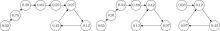
where α is the control parameter and when α ∈ [3.57, 4], the logistic map is in the chaotic state, n is the time index, and xn denotes the status value for the initial value after n − 1 iterations. The parameter α is 4. Using numerical simulation, we obtain three representative sequences whose initial values are 0.02, 0.65 and 0.03. As shown in Fig. 1, an infinite loop occurs after several iterations when the sequence value becomes 0.97, 0.42 or 0.12. Such a dynamical degradation phenomenon can result in the performance attenuation of digital chaos based processing, e.g. the chaos based cryptosystems become vulnerable to attack.[5, 6] Therefore, preventing the side-effects caused by the dynamical degradation is always a challenge to the chaos based cryptosystems.
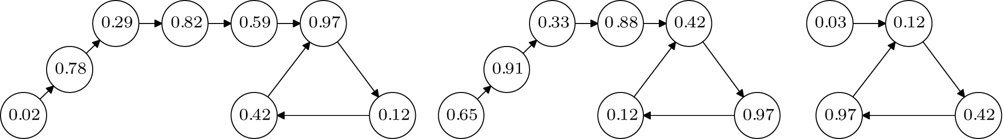 | Fig. 1. Degradation phenomenon of logistic map when the precision is 0.01. |
Five remedy methods are commonly used for preventing the dynamical degradation of digital chaos systems. (i) Using high finite precision, [7] which can slow down the speed of degradation with gradually increasing the number of iterations, but the degradation still exists; it is not really a fundamental solution for chaos systems’ degradation. (ii) Cascading multiple chaos systems.[8] This method can effectively prolong the cycle of orbit but often leads to a worse distribution. (iii) Switching multiple chaos systems, which can also weaken the degradation and extend the length of the chaotic sequence.[9, 10] But in this scheme the length of chaotic sequence is just a superposition of each chaotic sequence, therefore, the degradation phenomenon is still not alleviated. In addition, it is difficult to design a proper switch rule to preserve the properties of the system. (iv) Coupling different chaos systems, which is another method to reduce the degradation. As for this method, a proper chaos should be selected to avoid that the loss of system complexity exceeds the gain of performance improvements, otherwise it would lose the practicability. For example, a unidirectional coupling based hybrid method uses the three-dimensional (3D) Lorenz system to couple a one-dimensional (1D) logistic map.[11] Although the dynamical property of the logistic map is promoted, the complexity of the system is increased greatly. Using a continuous system to couple a discrete system is difficult in practical work because the Lorenz system costs more resources than the discrete-time chaos when they are implemented on the hardware.[12, 13] The computing speed will be pulled down as the continuous system requires a longtime period for computation. (v) Pseudo randomly perturbing the chaos system, [14] which can greatly improve the dynamical properties of digital chaos systems and has been proved to be better than the aforementioned methods.[15] Although the perturbation sources are also generated on digital devices in the existing perturbation algorithms, a good performance can be obtained as long as the proper perturbation method is confirmed. Furthermore, this method does not need any large scale system which makes it easy to implement. The perturbation objects include system parameter and sequence value, and the perturbation degree and interval can be managed so that there will be significant influence on the performance of the result. In this paper, a new parameter perturbation method for the tent map based on the Lyapunov exponent and Chebyshev map is proposed. The main contributions of this paper include that i) a novel perturbation principle and method for the Tent map are proposed and ii) the performance evaluation results and a case study are also given. The rest of the paper is organized as follows. In Section 2, the performance of the Tent map and Chebyshev map is analyzed and a perturbation method is proposed. Performance analysis results and a case study are given in Section 3. Finally, some conclusions are drawn Section 4.
Firstly, the analysis of the tent map and Chebyshev map are given in this section as they are both employed in the proposed perturbation method. The nonlinear tent map is a classical piecewise chaos system. It is defined as
where a is the control parameter. When α ≠ 0.5 and α belong to most parts of interval (0, 1), the system presents good pseudo-randomness. The output of the tent map is in the interval of (0, 1), which has the same invariant density distribution: ρ (xn) = 1. The Lyapunov exponent of the tent map is shown as follows:
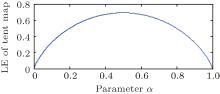
It can be seen that the Lyapunov exponent only depends on parameter a. From the research outcome of Ref. [16], it is known that a system is in a chaotic state when the Lyapunov exponent is positive, and the chaotic state keeps a high level when the Lyapunov exponent is high. Figure 2 is the Lyapunov exponent (LE) of tent map versus system parameter α . The Lyapunov exponent is positive in the whole domain of a. When a = 0.5, the tent map has the biggest Lyapunov exponent (i.e. ∼ 0.7), and when it is in the interval of (0.2, 0.8), the Lyapunov exponent is kept in a relatively high level (i.e., ∼ 0.5).
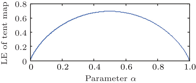 | Fig. 2. Lyapunov exponent (LE) of tent map versus parameter a. |
The Chebyshev map is another chaos system which is based on the trigonometric function. It is defined by

where β is the system parameter. When β ≥ 2, the Chebyshev map has good chaotic properties with mixture and ergodicity, and its Lyapunov exponent is positively correlated to the parameter β .[1] Let {yi} be the chaotic sequence generated by Eq. (4), the statistical property of the chaotic sequence can be achieved by the following steps: Firstly, the probability density of a chaotic sequence generated from the Chebyshev map can be generated as shown below.

Secondly, the mean of {yi} can be obtained on the basis of the following equation:

Equation (6) can be used to express the statistical property of the chaotic sequence. It indicates that the chaotic sequence generated by the Chebyshev map has good distribution characteristics as the mean of {yi} is 0. This feature is appropriate to use in the random number generating. In addition, the sequence value of the Chebyshev map ranges from − 1 to 1, which is broader than that of the tent map.
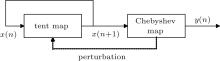
According to the properties of the tent map and Chebyshev map, a novel special perturbation method is proposed in this paper. It is shown in Fig. 3 where the tent map is the original pseudo-random number generator, and its iteration values are sent to the Chebyshev map for the post processing.
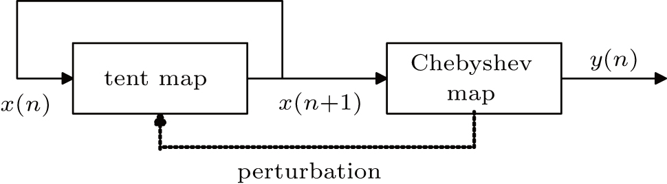 | Fig. 3. Perturbation method. |
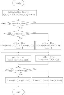
Specifically, figure 4 shows the flow chart of the proposed system, where a 1D matrix − P_ tent(1, i) is used to store the changing parameters of the tent map, x(1, i) is the sequence value of the tent map, y(1, i) is the final output of the proposed system. Assigned to the system are an initial value and an initial parameter, which are denoted by x(1, 1) and P_ tent(1, 1) respectively. As shown in Fig. 3, there are mainly two blocks in the proposed system. The first block is a tent map, and the other block is the post processing – parameter perturbation and transfer. All the chaotic values generated from the tent map are iterated once again through the Chebyshev for the post processing, that is, y(l, i) = cos(β · cos− 1(x(l, i + l))). The corresponding status values generated by the Chebyshev map are the final output. Suppose that δ is one of the final outputs, if δ falls into a range of (0.2, 0.5) or (0.5, 0.8), it will not only be used as the output value of the chaotic sequence but also sent back to the tent map to replace the original parameter a, then δ will be the parameter of the tent map in the next iteration. Otherwise, the parameter of the tent map in the last iteration is preserved for the next iteration. Therefore, the parameter of the tent map is always changed as long as the final output of the Chebyshev falls into an appropriate range.
 | Fig. 4. Flow chart of the proposed system. |
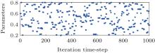
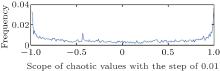
Figure 5 shows the changing parameters of the tent map in the first 1000 iterations. It can be seen that the parameter changes hugely and continuously after several iterations. The changing parameters of the tent map destroy the original chaos orbit, which greatly prohibits the short circle phenomenon from occurring. Moreover, the post processing reduces the correlation among the status values. Figure 6 is the frequency distribution of the chaotic sequence generated by the proposed system. The chaotic sequence has a ‘ U’ -shaped invariant density function, which is uniform except for two endpoints of − 1 and 1. For a fixed length sequence, the probability distributed in each sub interval will be reduced as the scope of the output values extends to (− 1, 1). In this way, the proposed perturbation method can enhance the resistance to frequency attack.
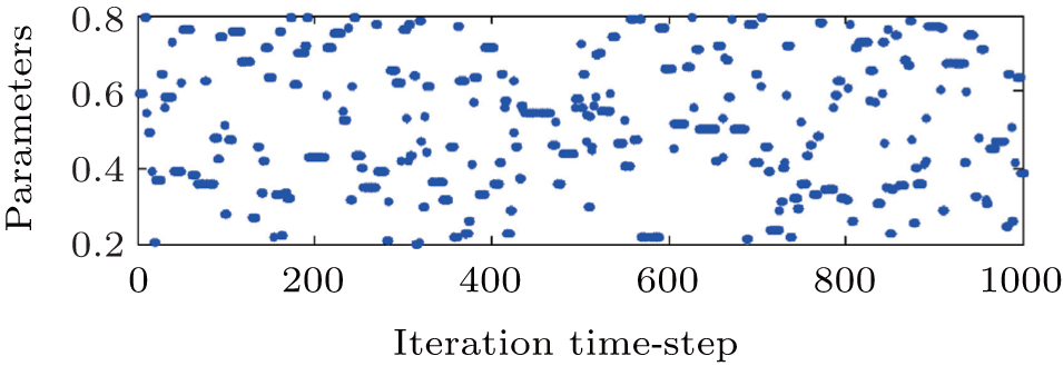 | Fig. 5. Changing parameter of the tent map. |
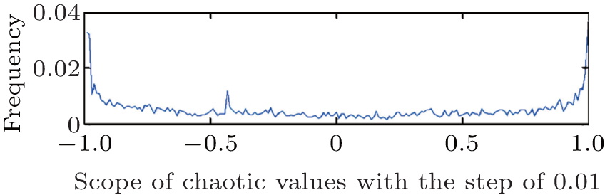 | Fig. 6. Frequency distribution of output sequence of the proposed perturbation system where the step is 0.01. |
Autocorrelation is used to describe the correlation between any two different values in one number sequence. The normalized autocorrelation function of an arbitrary ideal random sequence {yi} is
where ρ (y) is defined by Eq. (5) and the PSD represents the power spectral density. In addition, according to Golomb’ s postulate for a pseudo-random sequence, an ideal chaotic sequence should have an important characteristic: its autocorrelation should be a delta function.[17, 18]
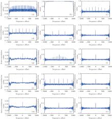
Figure 7 shows the autocorrelations of the sequences generated by different chaos systems. The three figures in each column from left to right are the distributions of the tent map, Chebyshev map and the proposed perturbation system, respectively. The precisions adopted by all the five rows are different ranging from 10− 4 to 10− 8. The three sequences have the same length of 1000, and the same initial value of 0.3. In addition, for the Chebyshev map and the proposed perturbation system, the parameter β is 6. According to Eq. (7) and the Golomb’ s postulate, it is easy to see that the autocorrelation of the proposed system has achieved an ideal state when the computation precision is 10− 5, i.e. the shape of autocorrelation is similar to a delta function. The autocorrelation of the tent map has no burrs until the computation precision runs up to 10− 7. In addition, the AC(m) of the tent map does not achieve 0 when m ≠ 0, which indicates that the chaotic sequence has a strong correlation. For the Chebyshev map, its AC(m) achieves an ideal state until the computation precision is 10− 8 as shown in Fig. 7(n). The ‘ threshold accuracy’ is defined as the time when the AC(m) of a sequence reaches the ideal state under the lowest computation precision. Figure 7 illustrates the AC(m)s of the Tent map, Chebyshev map and the proposed system under precisions ranging from 10− 4 to 10− 8. It is clear to see that the threshold accuracy of the proposed system is 10− 5, the threshold accuracy of the Chebyshev map is 10− 8 and the threshold accuracy of the Tent map is higher than 10− 8. Therefore, the proposed system has a lower threshold accuracy than the tent map and Chebyshev map, i.e. it has the better chaotic feature.
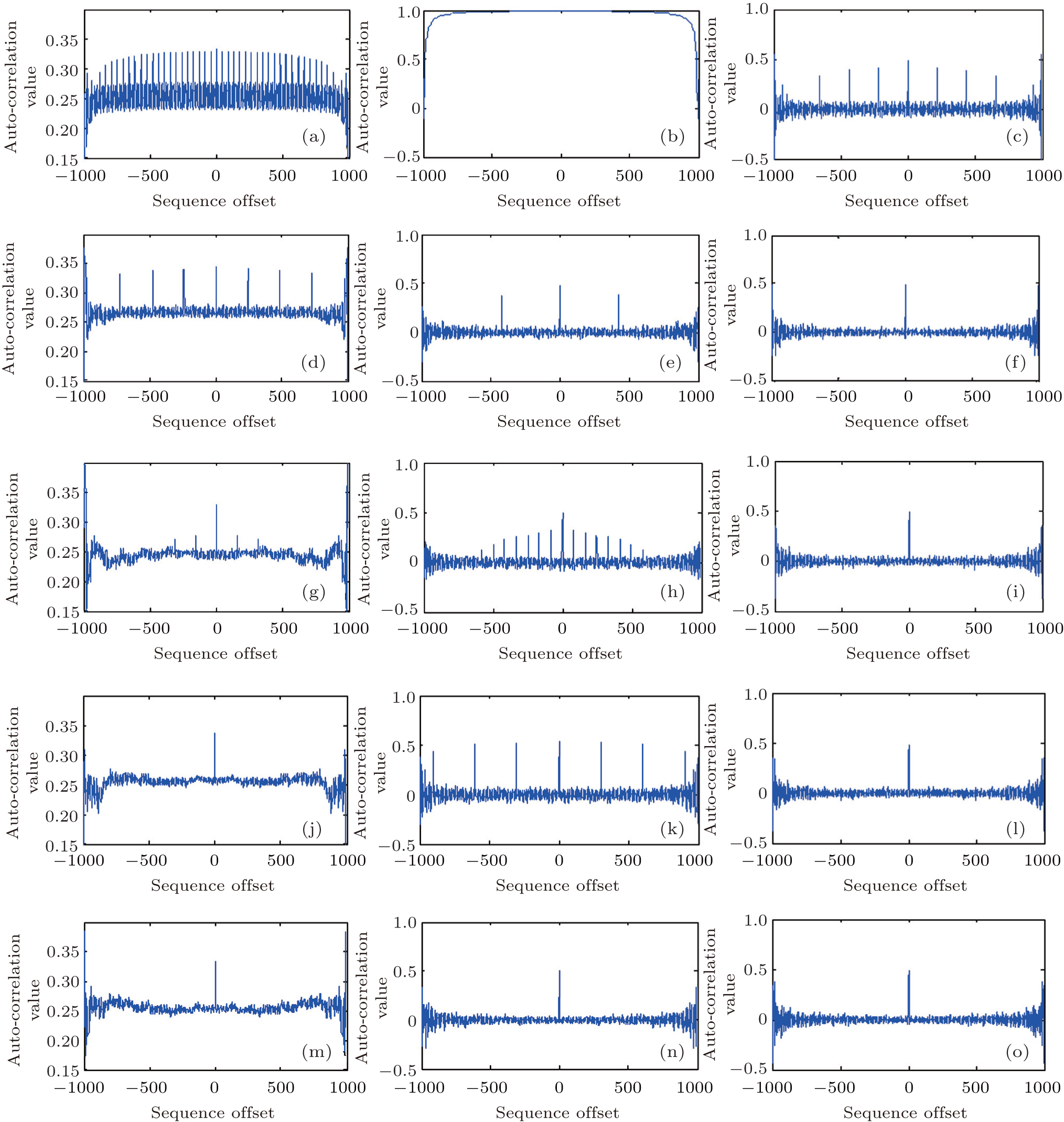 | Fig. 7. AC(m)s under the precisions ranging from 10− 4 to 10− 8: tent map (a), (d), (g), (j), (m); Chebyshev map (b), (e), (h), (k), (n); and the proposed system (c), (f), (i), (l), (o). |
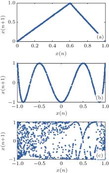
The shape converged by all the values of one chaotic sequence in the spatiotemporal domain is defined as the chaos attractor. Most of the chaos attractors always have some geometric shapes and the complexity of the attractors can reflect the confusion degree of the chaos system. Figure 8 presents the chaos attractors of the tent map, Chebyshev map and the proposed perturbation system. The three different attractors all consist of the chaotic sequences each with a length of 1000. As shown in Fig. 8 the tent map has a piecewise linear attractor, and the Chebyshev map has a cosine function attractor. Any orbit of the two systems can traverse the whole interval of their mapped values. Compared with the two simple maps, the proposed perturbation system has a better ergodicity as the shape of attractor is destroyed. It makes the generated sequence appear “ random” to the intruder. Thus the obvious correlation of neighbourhood is destroyed which enhances the security of the digital chaos system.
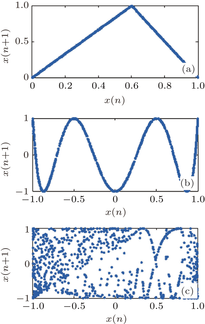 | Fig. 8. Chaos attractors of (a) tent map, (b) Chebyshev map, and (c) the proposed system. |
The approximate entropy is used to measure the complexity of the discrete time sequence. If the approximate entropy is too big, it will indicate that the sequence has a good complexity and stability. The test experiment is carried out by the following seven steps.
Step 1 A 1D discrete-time sequence with a length of N is given as {u(i), i = 1, … , N}, then rebuild it into an m-dimensional vector: Xi = {u(i), u(i + 1), … , u(i + m − 1)}, in which i = 1, 2, … , n, n = N − m + 1.
Step 2 Compute the distance between any two vectors Xi and Xj(j = 1, 2, … , N − m + 1, j ≠ i). The maximum absolute value of the corresponding elements between any two different vectors is defined as the distance that is described as

Step 3 Give a threshold value γ , normally in the interval of (0.2, 0.3). Count the number of dij which is less than γ × (SD), where SD is the standard value of the vector. Then the number is multiplied by 1/(N − m). The resulting number is denoted as 
Step 4 Transform 

Step 5m is added by one, repeat the four steps above. 

Step 6 The 


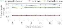
In this paper, the length of N is set to be 1000. Figure 9 shows the approximate entropies of the tent map, Chebyshev map and the proposed system. The x axis is the data precision P, e.g. the data precision is 10− 10 if p = 10. It can be seen that the approximate entropy of the proposed perturbation system (i.e. ∼ 1.8) is greater than those of the tent map (i.e. ∼ 0.55) and Chebyshev map (i.e. ∼ 1.5), which means that the parameter perturbation can not only greatly enhance the complexity of the tent map but also make it more complicated than that of the Chebyshev map. Moreover, the approximate entropy of the proposed perturbation system is almost invariable with computation precision, i.e. the approximate entropy is still high even if the data precision is low (e.g. P = 5). Therefore, the proposed method is robust to computation precision, i.e. the expected chaotic sequence can be obtained even with a low precision; therefore the computing cost can be reduced (especially for the embedded system implementation).
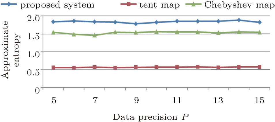 | Fig. 9. Approximate entropies of the tent map, Chebyshev map, and the proposed system. |
If the system parameter is fixed, when the initial value has a small change, the extent of change of the sequence value can reflect the system sensitivity to the initial value. In this experiment, the system parameter is fixed to be a = 0.6, the initial value is x0 = 0.3 and the change of initial value is 0.0000000001 (i.e., 10− 10). Figure 10 shows the output values of the original system and the modified system with a tiny change for the initial value. It can be seen that the output values of these two systems are completely different, e.g. after ∼ 20 times iterations, they begin to separate from each other. This shows that the proposed system maintains a high sensitivity to the initial value.
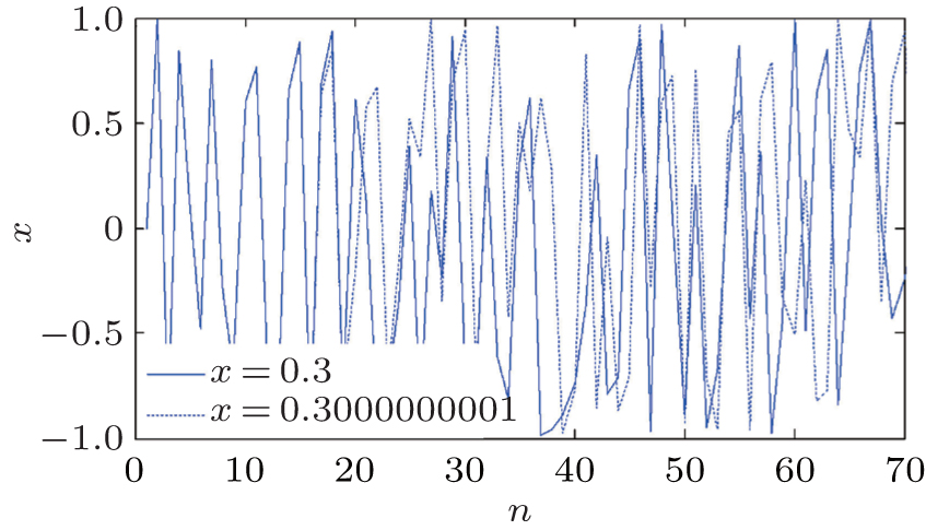 | Fig. 10. Two sequences for different initial values. |
The SP 800-22 is a statistical test consisting of 15 tests. It was developed to test the randomness of arbitrarily long binary sequences produced by cryptographic random or pseudorandom number generators.[19, 20] These tests focus on different types of non-randomness that could exist in a sequence. Each test is applied to the same sequence of n bits and gives a P-value, i.e. the probabilistic measure of the randomness of the sequence under test. If the significance level α is chosen to be 0.01 (common value of α in cryptography is about 0.01), then about 1% of the sequences are expected to be nonrandom.[6] A sequence passes a statistical test whenever the P-value ≥ α ; otherwise it fails. In this experiment, the length of a bit-sequence produced by the proposed system is 107 bits, which is longer than values obtained by the approaches of Refs. [6] and [20], i.e., 105 and 106, respectively. The results of testing a sequence’ s P-values are shown in Table 1. It can be seen that the proposed system passes all the tests and the produced sequence has a good pseudo-randomness.
| Table 1. SP 800-22 test results of the sequence produced by the proposed system. |
An image encryption experiment is designed by using the proposed perturbation system, where the generated chaotic sequence is employed to encrypt the image. Suppose that the size of the plain image is M × N, the encryption algorithm is defined as follows.
Step 1 Iterate the proposed system (M × N − 1) times, the corresponding chaotic sequence is

within a precision of 10− 15 where Si ∈ (− 1, 1).
Step 2 Transform the sequence Si as follows:


where the ‘ abs’ operation means taking the absolute value, while ‘ mod’ is the module operation. The ‘ uint8’ is compulsory conversion. The real numbers are transformed into the integers with the format of 8-bit unsigned binary. After the transform, the numbers in Si can be used to encrypt the plain image.
Step 3 Using the improved numbers in Si to execute the bit-xor operation with all the pixels one by one from left to right, top to bottom.
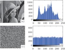
Using this encryption algorithm, the plain image can be encrypted very well. A standard Lena image is used to evaluate the performance of the proposed encryption algorithm. The original Lena image with a size of 256 × 256 is shown in Fig. 11(a) and the corresponding histogram is shown in Fig. 11(b). Figure 11(c) is the encrypted image with the encryption key x0 = 0.3 (i.e. the initial value of the proposed perturbation system), and its histogram is shown in Fig. 11(d). From these figures, it can be seen that the histogram of the encrypted image is fairly uniform and is significantly different from the original image as the image pixels of the encrypted image are distributed uniformly.
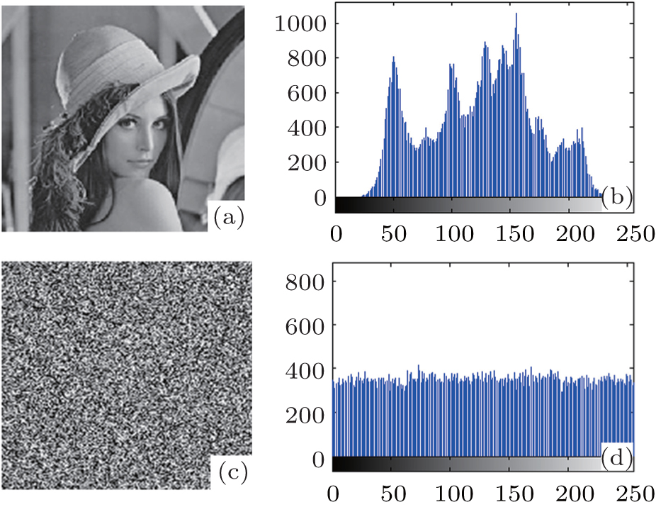 | Fig. 11. Image encryption results: ((a) and (b)) Lena image and histogram, ((c) and (d)) encrypted image and histogram. |
In addition, an experiment is carried out to test the entropy and the correlation between two adjacent pixels in vertical, horizontal, and diagonal directions of the cipher image. Table 2 shows the corresponding performance tests and comparisons. The same image of Lena by using the approaches of Refs. [1], [3], [21], and [22] are encrypted by their corresponding algorithms for 1, 2, 2, and 3 rounds, respectively. However, this method only needs one round of bit-xor encryption through the proposed system. But the cipher image achieves a good performance in correlation coefficient and entropy tests as well. In addition, from the results shown in Table 2, we can see that the time consumption of this case is the smallest in all the approaches. Therefore, the proposed system can be used in cryptography.
| Table 2. Comparisons of cipher image among different approaches. |
In this paper, a novel parameter perturbation method for the tent map is proposed. Based on the Lyapunov exponent and Chebyshev map, the chaotic properties of the proposed system are hugely improved compared with those from the tent map and the Chebyshev map. This perturbation method can weaken the phenomenon of strong correlation caused by the finite precision, reduce the sequence’ s dependence on the perturbation signal and effectively compensate for the dynamics degradation of the digital chaos system. The theoretical analysis, performance tests and experimental results show that the proposed method can produce a pseudo-random sequence with good cryptographic properties, which has a good application potential in the fields of confidential communication.
| 1 |
|
| 2 |
|
| 3 |
|
| 4 |
|
| 5 |
|
| 6 |
|
| 7 |
|
| 8 |
|
| 9 |
|
| 10 |
|
| 11 |
|
| 12 |
|
| 13 |
|
| 14 |
|
| 15 |
|
| 16 |
|
| 17 |
|
| 18 |
|
| 19 |
|
| 20 |
|
| 21 |
|
| 22 |
|