


Time-domain nature of group delay
[Wang Jian-Wu†a), b)  , Feng Zheng-He
a) ]
, Feng Zheng-He|
|


†Corresponding author. E-mail: wangjianwuradar@163.com
*Project supported by the National Basic Research Program of China (Grant No. 2013CB329002) and the National Natural Science Foundation of China (Grant No. 61371012).
The characteristic of group delay is analyzed based on an electronic circuit, and its time-domain nature is studied with time-domain simulation and experiment. The time-domain simulations and experimental results show that group delay is the delay of the energy center of the amplitude-modulated pulse, rather than the propagation delay of the electromagnetic field. As group velocity originates from the definition of group delay and group delay is different from the propagation delay, the superluminality or negativity of group velocity does not mean the superluminal or negative propagation of the electromagnetic field.
Group delay τ g is defined as the derivation of the phase response ϕ of a device or medium with respect to frequency f, and is given by

In engineering, group delay is always regarded as the envelope delay of a signal.[1– 7] Corresponding with the group delay, group velocity vg is defined to describe the propagation velocity of the envelope, and is given by[8]

where l is the travel distance of the signal and k is the wave number.
As research on group delay continues, the superluminality of group velocity is realized in electronic circuits, [9– 11] optical fibers, [12– 14] photonic crystals, [15– 17] and some special medium.[18, 19] The superluminality and negativity of group velocity raise a question: does the superluminality of group velocity not conform to the special relativity or does its negativity disobey the casualty? According to the discussion in Refs. [2]– [4], the superluminality and negativity of group velocity are caused by the interference between different frequency components. Owing to the interference, distortion occurs in the front or other regions of the pulse. In a word, all of the research holds a common opinion that the superluminality and negativity of a pulse are caused by the distortion, and the propagation of the front (or initial point) of the pulse cannot exceed the velocity of light. Then, another question rises: if group delay is not the delay of the front (or initial point) of the pulse, which delay does it characterize? In the existing research, none of them have paid any attention to the question.
At present, there is no such theory which can be utilized to analyze the time-domain characteristics of a pulse signal. The time-domain characteristics of a pulse signal are studied by observing its waveform in an oscilloscope only. Therefore, time-domain simulation and experiment are the only methods to study the time-domain nature of group delay based on pulse signals for the moment. Based on the discussion above, this paper is organized as follows. The characteristic of group delay is analyzed based on a simple electronic circuit with negative group delay in the second part; then, time-domain simulations are carried out to find the time-domain parameter whose delay may be consistent with group delay; when the time-domain parameter is found, further simulations and experiments are conducted to validate the consistency between group delay and the delay of the time-domain parameter.
By observing the superluminal devices, it can be found that there are capacitances and inductances or several travelling paths in all of the devices. The transmission of signal can be described by the signal flow graph in the device with capacitances and inductances.[20] For example, the simple electronic circuit with an inductance L and two resistances R0, 1 can be described by the signal flow graph in Fig. 1. According to the signal flow graph, the output signal is the superposition of the signals travelling in different paths. As a result of their superposition, the output signal is distorted. In other words, the capacitance, the inductance and the multi-path effect can be comprehended as a reformer of the input signal. Therefore, the group delay of a device with capacitance, inductance or multi paths is composed of two parts:
(i) the propagation delay of the electromagnetic field; (ii) the reformulating delay caused by the reformulating distortion.
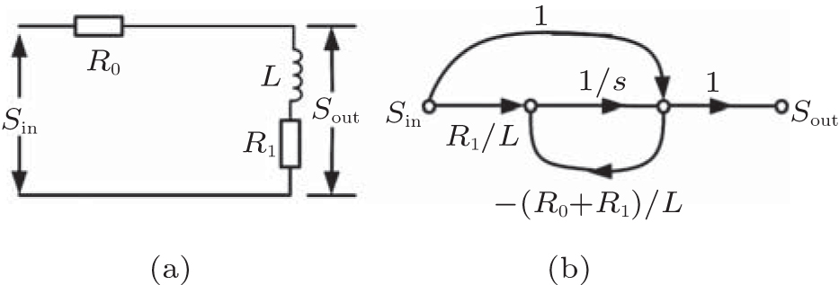 | Fig. 1. (a) Circuit for the example and (b) its signal flow graph. |
In free space, group delay is dominated by the propagation delay of the electromagnetic field. In a resonant device, such as a filter, group delay is dominated by the reformulating delay. When the reformulating delay is negative and small enough, group delay will be negative.
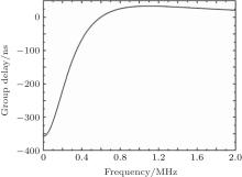
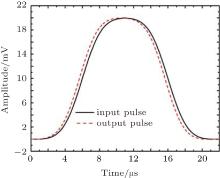
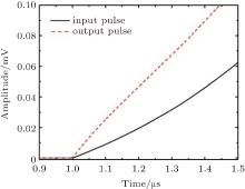
Figure 2 shows the group delay of the circuit in Fig. 1 with L = 10 μ H, R0 = 50 Ω , and R1 = 20 Ω . As shown in Fig. 2, the group delay is negative in the low-frequency zone. Figure 3 shows the waveforms when a pulse passes through the circuit. In order to compare the two waveforms, the output signal is amplified by multiplying it with 3.5. As shown in Fig. 3, the output pulse precedes the input pulse on the whole. However, when the initial area of the two pulses is amplified enough as shown in Fig. 4, the front of the output pulse is distorted and its initial point does not precede that of the input pulse. Therefore, the group delay is not the propagation delay of the electromagnetic field. The question about which delay characterizes the group delay needs studying.
 | Fig. 2. Group delay of the circuit in Fig. 1. |
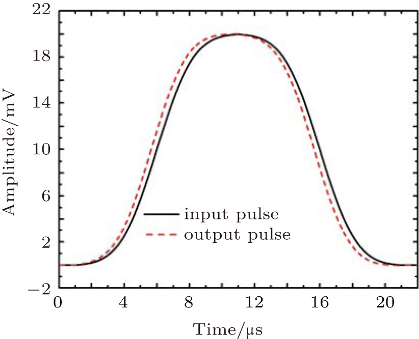 | Fig. 3. Waveforms of the input and output signals. |
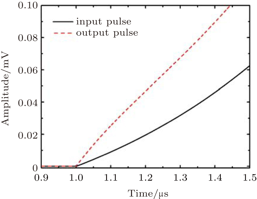 | Fig. 4. Amplified view in the initial area. |
In a broad sense, there are two kinds of envelopes: the amplitude modulation envelope and the phase modulation envelope. However, there is a problem in phase modulated signals: the signal can be described in different forms. For example, a chirp pulse with a modulated bandwidth of γ T can be described by
where Δ f0 = γ t0; γ is a constant; τ 0 is the initial point of the pulse; T is the width of the pulse. Therefore, both the carrier and envelope of the chirp pulse are not unique. According to the definition of group delay, the group delay of a specific device is determined by the carrier frequency. Therefore, the phase modulation cannot be used to find the time-domain nature of group delay. In other words, the envelope referred to in this paper is the envelope of the amplitude modulation only.
As analyzed in Section 2, the group delay is composed of the propagation delay and the reformulating delay. Owing to the reformulating of the envelope, the waveform of the pulse is distorted. In other words, when group delay is utilized to describe the delay of a pulse with a relatively narrow bandwidth, the time-domain parameter which is consistent with group delay will be related to the waveform of the envelope. Among the time-domain parameters, such as the peak of the envelope, the rising (falling) time of the envelope and the energy of the envelope, the concept of energy is related to the waveform of the envelope, and the others are related to the value of a single point only. Therefore, we try to find the time-domain parameter which is consistent with group delay based on the concept of energy in the following.
If the width of a pulse signal is T and the integral time T′ > T, the energy of the pulse signal is defined as

where A(t) is the envelope of the pulse signal. Then, a relative energy η is defined as the criterion for the measurement of time delay in time domain. η is given by

where E′ is the energy of the signal when there is no intact pulse in the integral time. The following are the steps to search for the time-domain parameter which is consistent with group delay by digital means:
Step 1 digitalizing both the input signal and output signal simultaneously with a sampling period Ts. The sampling period Ts determines the time resolution of the measured delay. In the following simulations of this paper, Ts is set to be 1 ns;
Step 2 demodulating the signals by squaring the modulated signals and averaging the signals with a length of Nd points. Nd is given by
where f0 is the carrier frequency and “ round()” rounds the element in the bracket to the nearest integers;
Step 3 determining the time ξ out when the relative energy of the output signal reaches η and the time ξ in when the relative energy of the input signal reaches η ;
Step 4 calculating the time delayτ by

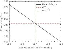
For a pulse, it is the complex superposition of many tones. In many circumstances, the group delay of a device is not a constant in a certain bandwidth, which means that different tones experience different envelope delays. As a consequence, the delay obtained by the time-domain method is affected by the bandwidth of the testing signal. In order to suppress the error caused by the bandwidth of the testing signal, the simulation is carried out at the central frequency of a third-order Butterworth filter, where the group delay is approximate to a constant in a narrow band. The simulations of this paper are conducted in MATLAB. The time delay τ and group delay τ g are both shown in Fig. 5 when a rectangle-modulated pulse passes through the third-order filter. The central frequency of the filter is 20MHz and the bandwidth is 2 MHz. The width of the pulse is 50 μ s. As shown in Fig. 5, the time delay obtained by the time-domain method is equal to the group delay at η = 0.5. In this paper, the point where E′ = E/2 is named the energy center of the signal. Therefore, the energy center can be taken as the candidate of the time-domain parameter which is consistent with group delay.
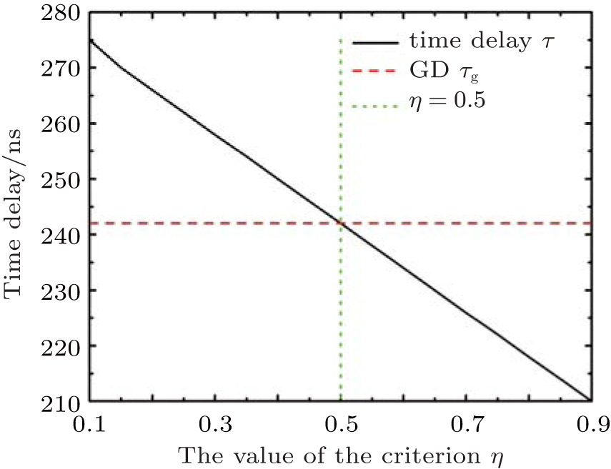 | Fig. 5. Measured time delay by the time-domain method with different criteria. |
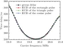
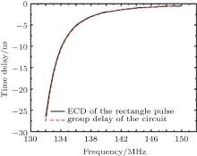
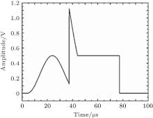
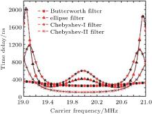
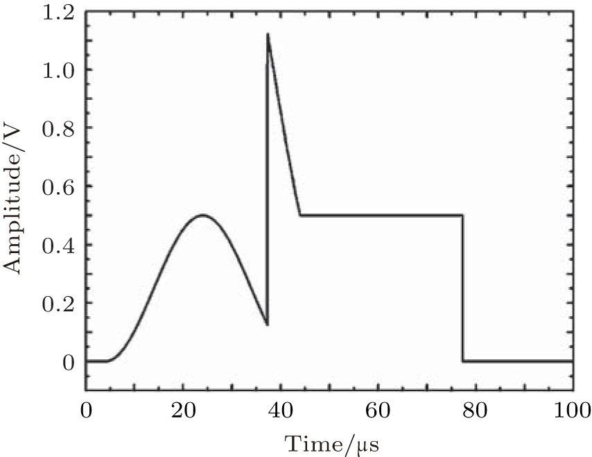
The energy center delays (ECDs) of the rectangle-modulated pulse, the triangle-modulated pulse and the cosine-modulated pulse are calculated for further demonstration in the whole pass band of the filter. The results are shown in Fig. 6 and the widths of the pulses are all 50 μ s. Besides, simulations with the circuit of negative group delay are also performed to demonstrate the consistence between group delay and ECD. The circuit of negative group delay is shown in Fig. 7, and figure 8 is the ECD of the rectangle-modulated pulse when it passes through the circuit. An irregular pulse is also utilized to demonstrate the consistence. Figure 9 shows the envelope of the irregular pulse, and figure 10 displays the ECDs of the irregular pulse when it passes through a Butterworth filter, an ellipse filter, a Chebyshev-I filter and a Chebyshev-II filter. All the filters are the third-order filters each with a bandwidth of 2 MHz. In Fig. 10, the black solid lines represent the group delays of the filters and the red dashed lines refer to the ECDs of the irregular pulse when it passes through the filters. As shown in Figs. 6, 8, and 10, there are slight differences between the ECDs and the group delays. Three factors may be responsible for the difference: 1) the time resolution; 2) the bandwidth of the testing signal; 3) the ripples after demodulation. Despite the slight differences, the ECD curves are consistent with the curves of group delays as a whole. Then, negative group delay can be explained reasonably: because of the reformulating delay, the power center of the output pulse precedes that of the input pulse with a relatively narrow bandwidth.
 | Fig. 6. Group delays and ECDs in the pass-band of the third-order Butterworth filter. |
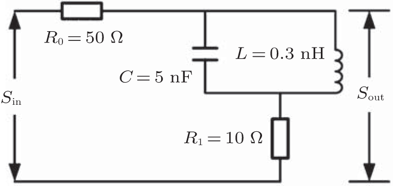 | Fig. 7. Circuit of negative group delay. |
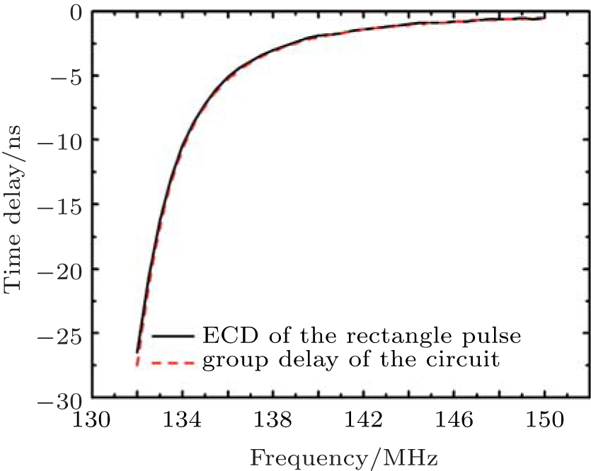 | Fig. 8. The ECD and group delay of the circuit shown in Fig. 7. |
 | Fig. 9. Envelope of the irregular pulse. |
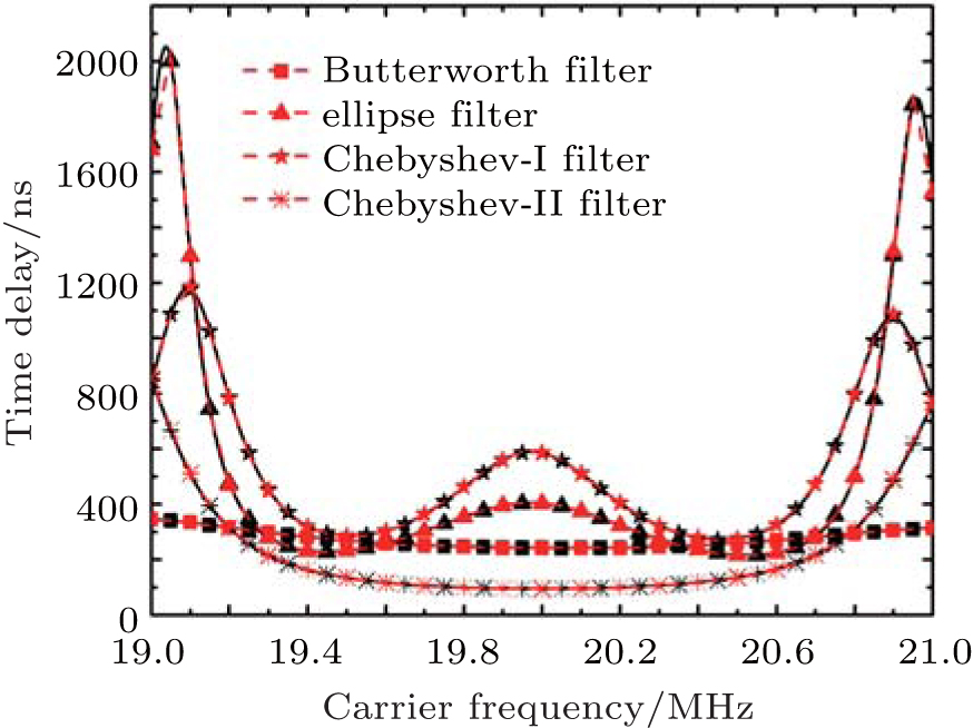 | Fig. 10. The ECDs of the irregular pulse and the group delays of the filters. |
The experiment is done with a filter to validate the time-domain interpretation of group delay. The block diagram of the experiment is shown in Fig. 11. As shown in Fig. 11, the measured delay is the relative delay of port-2 with respect to the delay of port-1. In the experiment, the sampling rate of the oscilloscope is set to be 1 GHz, and the length of data is assumed to be 65536 Bytes. For the non-rectangle-modulated pulse, it can be comprehended as a further amplitude modulation added to the rectangle modulation. Because of the further modulation, the bandwidth of the pulse is broadened. Consequently, the possible error caused by the bandwidth of the testing signal increases when the time width of the pulse is fixed. Therefore, rectangle modulation is chosen in the experiment. An Agilent N5182A is utilized to generate the rectangle pulses with a period of 80 μ s and a width of 10 μ s.
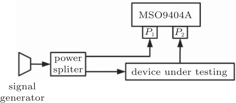 | Fig. 11. Diagram of the experiment. |
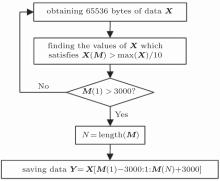
In the measurement of the relative ECD, an intact pulse must be contained in the data block for calculation. Therefore, a simple algorithm shown in Fig. 12 is utilized in data capturing to make sure that the condition is satisfied.
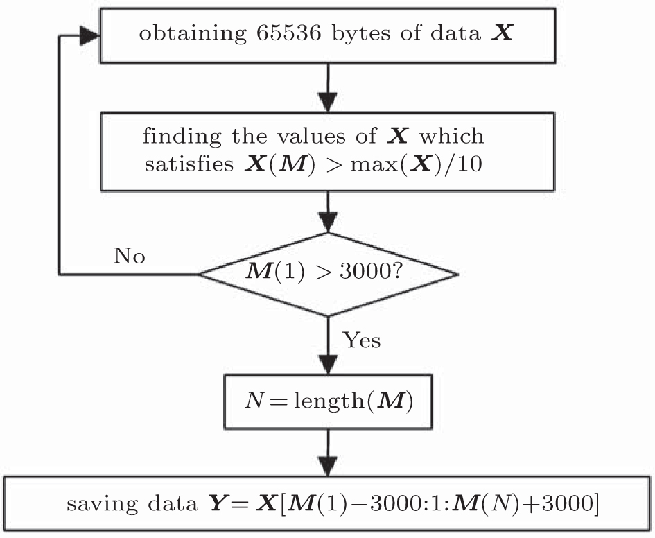 | Fig. 12. Algorithm for data capturing. |
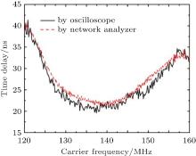
The bandwidth of the filter under testing is 40 MHz and the central frequency is 140 MHz. In order to validate the time-domain interpretation, the relative ECD is compared with the relative group delay obtained by the network analyzer N5071B. The procedure for obtaining the ECD is the same as that presented in Section 3 with η = 0.5. The results are shown in Fig. 13. As shown in Fig. 13, the result obtained by the oscilloscope is consistent with that obtained by the network analyzer. Therefore, the time-domain interpretation of group delay is reasonable.
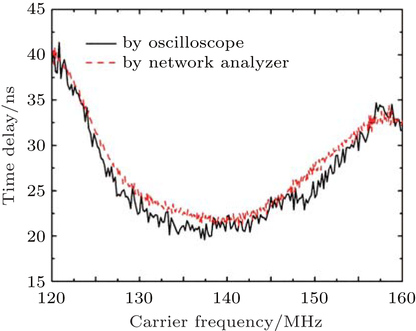 | Fig. 13. Measured results of time delay versus carrier frequency for a filter. |
In this paper, we study the time-domain nature of group delay by the time-domain simulations and experiment. Our research reveals that the group delay is consistent with the delay of the energy center (ECD) of the amplitude-modulated pulse. With the time-domain explanation, negative group delay can be explained reasonably: because of the reformulating delay, the power center of the output pulse precedes that of the input pulse with a relatively narrow bandwidth. However, since the simulations and experiments study specific structures, the conclusion needs to be further studied theoretically.
Based on the time-domain study, the controversy over the superluminality or negativity of group velocity can be clarified. As group delay is defined in frequency domain, its time-domain nature is unknown. Owing to its time-domain nature being unknown, group delay is confused with the concepts of the propagation delay. By studying the time-domain nature of group delay, the difference between group delay and propagation delay is revealed. As group delay is different from the propagation delay, neither the superluminality nor negativity of group velocity defies the special relativity or casualty.
| 1 |
|
| 2 |
|
| 3 |
|
| 4 |
|
| 5 |
|
| 6 |
|
| 7 |
|
| 8 |
|
| 9 |
|
| 10 |
|
| 11 |
|
| 12 |
|
| 13 |
|
| 14 |
|
| 15 |
|
| 16 |
|
| 17 |
|
| 18 |
|
| 19 |
|
| 20 |
|