Singular and non-topological soliton solutions for nonlinear fractional differential equations
[Guner Ozkan† ]
]
]
|
|


†Corresponding author. E-mail: ozkanguner@karatekin.edu.tr
In this article, the fractional derivatives are described in the modified Riemann–Liouville sense. We propose a new approach, namely an ansatz method, for solving fractional differential equations (FDEs) based on a fractional complex transform and apply it to solve nonlinear space–time fractional equations. As a result, the non-topological as well as the singular soliton solutions are obtained. This method can be suitable and more powerful for solving other kinds of nonlinear fractional FDEs arising in mathematical physics.
Fractional differential equations are the generalizations of classical differential equations with integer orders. In recent years, fractional differential equations have played an important role in different research areas such as mechanics, engineering, signal processing, stochastic dynamical system, plasma physics, electricity, electrochemistry, biology, control theory, systems identification, economics and finance.[1– 4]
Finding approximate and exact solutions to the fractional differential equations is an important task. Many powerful and reliable methods have been proposed to obtain the exact solutions of fractional differential equations. For example, these methods include the (G′ /G)-expansion method, [5– 7] the first integral method, [8– 10] the fractional sub-equation method, [11– 13] the exp-function method, [14– 16] the fractional functional variable method, [17, 18] the fractional modified trial equation method, [19] Kudryashov method, [20, 21] ansatz method, [22] and so on.
The theory of solitons is one of the very important areas of research in ocean dynamics, optics, plasma physics, fluid dynamics, semiconductors, and engineering. In these areas, the study of solitary waves attracts a lot of attention. Therefore, it is important to focus on solitary waves in a detailed manner from a mathematical point of view. Biswas et al. obtained optical solitons and soliton solutions with higher-order dispersion by using the ansatz method.[23– 25] This method was used by many authors.[26– 31] But, applications of this method are rather rare in the nonlinear fractional differential equations.
The rest of this paper is organized as follows: In Section 2, we describe the modified Riemann– Liouville derivative and explain how we can convert fractional differential equations into integer-order differential equations. In Sections 3 and 4, we apply this method to establish the exact solutions for the space– time fractional Boussinesq equation and the space– time fractional (2+ 1)-dimensional breaking soliton equations and to employ a variety of exact solutions to determine non-topological soliton solutions and singular soliton solutions. Conclusions are presented in Section 5.
Fractional calculus theory is almost more than two decades old in the literature. There are several approaches to the generalization of the notion of differentiation to fractional orders, e.g., Riemann– Liouville, Grü nwald– Letnikow, and Caputo.[32, 33] But the first major contribution to give proper definition is due to Jumarie’ s modified Riemann– Liouville derivative[34, 35] as shown below.
Definition 1 Assume that f : R → R, x → f (x) denotes a continuous (but not necessarily differentiable) function. The modified Riemann– Liouville derivative of order α is defined by the expression[36]

in which Γ (· ) is the Gamma function defined by[37]
or

It imposes advantages of fast convergence, higher stability, and higher accuracy to derive different types of numerical algorithms.
Definition 2 The Mittag– Leffler function with two parameters is defined as[38]

this function is used to solve fractional differential equations as the exponential function in integer order systems.
We list some important properties for the modified Riemann– Liouville derivative as follows:
Property 1

Property 2

Property 3

where a and b are constants.
We consider the following general nonlinear FDEs of the type

where 

By using the fractional complex transform we can convert fractional differential equations into integer-order differential equations
where k and c are nonzero arbitrary constants. Also, by using the chain rule
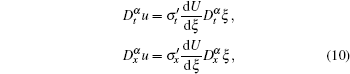
where 


Substituting Eq. (9) with Eq. (5) and Eq. (10) into Eq. (8), we can rewrite Eq. (8) in the following nonlinear ordinary differential equation (ODE);

where Q is a polynomial in U(ξ ) and its total derivatives U′ , U″ , U‴ , … , such that

If possible, we should integrate Eq. (11) term-by-term one or more times.
The first equation is called the space– time fractional Boussinesq equation which has the form[42]
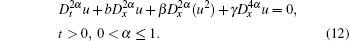
Here γ = const > 0 is the dispersion parameter depending on the compression and rigidity characteristics of the material, β = const is the coefficient controlling nonlinearity, u(x, t) is the vertical deflection, and the quadratic nonlinearity (u2)xx accounts for the curvature of the bending beam. α is a parameter describing the order of the fractional time and space derivative.
The bright and singular soliton solutions to Eq. (12) will be obtained with the help of the ansatz method.[43, 44] In order to solve Eq. (12), we use the following transformations,

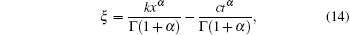
where k and c are non-zero constants.
Substituting Eq. (14) with Eqs. (5) and (10) into Eq. (12), this equation (Eq. (12)) reduced into an ODE

where “ U′ ” = dU /dξ . By integrating twice and setting the constants of integration to be zero, we obtain

The solitary wave ansatz for the bright (non-topological) 1-soliton solution, i.e., the hypothesis, is[45, 46]

where
Here, A, c, and k are nonzero arbitrary constants. The unknown p will be determined during the course of derivation of the solutions of Eq. (1).
Therefore from Eqs. (17) and (18), it is possible to get
and

Thus, substituting the ansatz Eqs. (17)– (20) into Eq. (16), yields
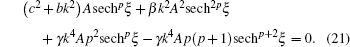
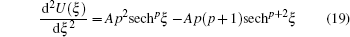
Now, from Eq. (21), equating the exponents p + 2 and 2p leads to

From Eq. (21), setting the coefficients of sechp+ 2ξ and sech2pξ terms to zero, we obtain

by using Eq. (22), we have

We find, from setting the coefficients of sechpξ terms in Eq. (21) to zero

also we get

From Eq. (26) it is important to note that

Thus, the 1-soliton solution of Eq. (12) is given by
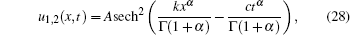
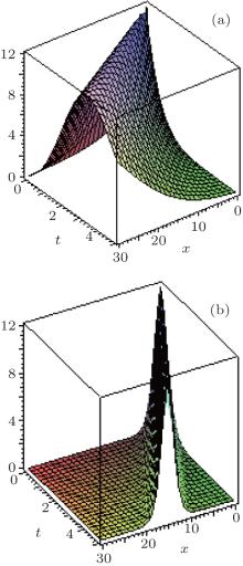
where A is given by Eq. (24) and c is given by Eq. (26). Also, the constraint condition is shown in Eq. (27). The evolution of exact solution for Eq. (28) with α = 0.5 and α = 1.0 is shown in Fig. 1.
 | Fig. 1. The exact solution for Eq. (28) with α = 0.5 (a) and α = 1 (b) respectively, when k = 1, γ = − 2, β = − 1, b = − 1. |
For singular solitons, the starting hypothesis is given by[47– 49]

where

where A, k, and c are nonzero arbitrary constants. The unknown p will be determined during the course of derivation of the solutions of Eq. (16). Equation (29) and its derivatives gives

and

Substituting Eqs. (29)– (32) into Eq. (16), we have

Similarly, from Eq. (33), equating the exponents p + 2 and 2p leads to

and

From Eq. (33), setting the coefficients of cschp+ 2ξ and csch2pξ terms to zero, we obtain

by using Eq. (35) and after some calculations, we have
We find, from setting the coefficients of cschpξ terms in Eq. (33) to zero

also we get

From Eq. (39) it is important to note that

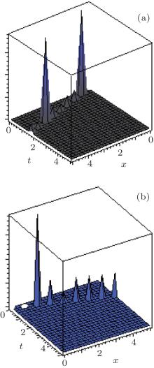
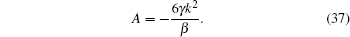
Thus, the singular soliton solution of Eq. (12) is given by
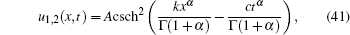
where A is given by Eq. (37), c is given by Eq. (39) and the constraint condition is shown in Eq. (40). The evolution of the exact solution for Eq. (41) with α = 0.5 and α = 1.0 is shown in Fig. 2.
 | Fig. 2. The exact solution for (41) with α = 0.5 (a) and α = 1 (b) respectively, when k = 1, γ = − 2, β = − 1, b = − 1. |
We consider the space– time fractional (2+ 1)-dimensional breaking soliton equations[50]


where 0 < α ≤ 1. In Ref. [50], Wen and Zheng applied the fractional sub-equation method to construct exact solutions of these equations. Equations (42) have been discussed in Ref. [51] using three different types of method, namely, the (G′ /G)-expansion method, the functional variable method, and the exp-function method. When α = 1, equations (42) are called the (2+ 1)-dimensional breaking soliton equations and some periodic wave solutions, non-traveling wave solutions, and Jacobi elliptic function solutions were found in Refs. [52]– [55].
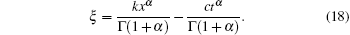
Now, we introduce the following transformations


where k, w, and c are non-zero constants.
Substituting Eq. (44) with Eqs. (5) and (10) into Eq. (42), equations (42) can be reduced into an ODE

where “ U′ ” = dU / dξ and “ V′ ” = dV/dξ .
Integrating the second equation in the system and ignoring constants of integration we obtain

Substituting Eq. (46) into the first equation of the system we find

Integrating Eq. (47) and ignoring constants of integration, we find

Substituting the ansatz [Eqs. (17)– (20)] into Eq. (48), yields
Now, from Eq. (49), equating the exponents p + 2 and 2p leads to

From Eq. (49), setting the coefficients of sechp+ 2ξ and sech2pξ terms to zero, we obtain,

by using Eq. (50) and after some calculations, we have

We find, from setting the coefficients of sechpξ terms in Eq. (49) to zero

also we get

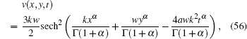
Thus, the non-topological soliton solution of Eq. (42) is given by

and from Eq. (46) we get
Substituting Eqs. (30)– (33) into Eq. (48), we have
Similarly, from Eq. (57), equating the exponents p + 2 and 2p we obtain p = 2. From Eq. (57), setting the coefficients of cschp+ 2ξ and csch2pξ terms to zero, we obtain

after some calculations, we have

We find, from setting the coefficients of cschpξ terms in Eq. (57) to zero

also we get

Thus, the 1-soliton solution of Eq. (42) is given by
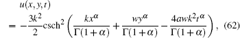
and
In this paper, we studied the non-topological and singular soliton solutions of nonlinear differential equations with fractional order. As a result, two types of soliton solutions for them have been successfully found. There are constraint conditions that must hold in order for the solitons to exist. The ansatz method was effectively used to achieve the goal set for this work. We have predicted that fractional complex transform with the help of the ansatz method can be extended to solve many systems of nonlinear fractional partial differential equations in mathematical and physical sciences.
| 1 |
|
| 2 |
|
| 3 |
|
| 4 |
|
| 5 |
|
| 6 |
|
| 7 |
|
| 8 |
|
| 9 |
|
| 10 |
|
| 11 |
|
| 12 |
|
| 13 |
|
| 14 |
|
| 15 |
|
| 16 |
|
| 17 |
|
| 18 |
|
| 19 |
|
| 20 |
|
| 21 |
|
| 22 |
|
| 23 |
|
| 24 |
|
| 25 |
|
| 26 |
|
| 27 |
|
| 28 |
|
| 29 |
|
| 30 |
|
| 31 |
|
| 32 |
|
| 33 |
|
| 34 |
|
| 35 |
|
| 36 |
|
| 37 |
|
| 38 |
|
| 39 |
|
| 40 |
|
| 41 |
|
| 42 |
|
| 43 |
|
| 44 |
|
| 45 |
|
| 46 |
|
| 47 |
|
| 48 |
|
| 49 |
|
| 50 |
|
| 51 |
|
| 52 |
|
| 53 |
|
| 54 |
|
| 55 |
|