Yamgoué Serge Bruno, Deffo Guy Roger, Tala-Tebue Eric, Pelap François Beceau. Exact transverse solitary and periodic wave solutions in a coupled nonlinear inductor–capacitor network. Chinese Physics B, 2018, 27(9): 096301
Permissions
Exact transverse solitary and periodic wave solutions in a coupled nonlinear inductor–capacitor network
Yamgoué Serge Bruno1, †, Deffo Guy Roger2, Tala-Tebue Eric3, Pelap François Beceau2
Department of Physics, Higher Teacher Training College Bambili, the University of Bamenda, P.O. Box 39 Bamenda, Cameroon
Unité de Recherche de Mécanique et de Modélisation des Systèmes Physiques (UR-2MSP), Faculté des Sciences, Université, de Dschang, BP 69 Dschang, Cameroun
Department of Telecommunication and Network Engineering, Fotso Victor University Institute of Technology, The University of Dschang, P.O. Box 134, Bandjoun, Cameroon
Through two methods, we investigate the solitary and periodic wave solutions of the differential equation describing a nonlinear coupled two-dimensional discrete electrical lattice. The fixed points of our model equation are examined and the bifurcations of phase portraits of this equation for various values of the front wave velocity are presented. Using the sine-Gordon expansion method and classic integration, we obtain exact transverse solutions including breathers, bright solitons, and periodic solutions.
The responses of nonlinear dispersive systems and their applications are fascinating subjects that are currently at the forefront of research in nonlinear optics,[1–4] plasma physics,[5,6] biology,[7] atomic chains,[8–11] Fermi–Pasta–Ulam lattices,[12–14], crystals,[15–19] and discrete electrical transmission lines[20–27] to mention just a few. Depending on the fields, several elements are at the origin of the nonlinear and dispersive character of these systems. In the case of electrical transmission lines (NLTL), for example, nonlinear and dispersion effects are introduced by nonlinear capacitors and linear inductors, respectively.
The combined effects of these two phenomena are capable of generating solitary waves in the system. The energy of such waves is localized in space and they are extremely stable during their propagation.[28] Several types have been studied. These solutions exist on several forms[29–32] and are shape-preserving in the nonlinear dispersive media through which they are propagated. They are very significant in diverse fields of physics and engineering. In modern textile engineering, for instance, non-linear differential-difference equations with soliton solutions are often used to describe some phenomena arising in heat/electron conduction and flow in carbon nanotubes.[33] Thus, soliton solutions and their interactions are theoretically investigated in various nonlinear evolutions equations such as the coupled KdV equations with variable coefficients,[34] the (2 + 1)-dimensional generalized fifth-order KdV equation,[35] the modified Zakharov–Kuznetsov equation,[36] the standard nonlinear Schrodinger equation and its extended forms,[37–41] the (2 + 1)-dimensional Ito equation,[42] the Kadomtsev–Petviashvili equation and its B-type,[43–45] to name just a few. There is equally a great deal of interest devoted to experimental investigations on solitons. This is conspicuously illustrated, for example, by the very recent paper by Liu et al.[46] and the large number of references therein on similarly works.
In the literature, many powerful methods have been developed by mathematicians and physicists to tackle the complexity of these model equations. Most of those methods have in common the fact that they assume the solutions in the form of an expansion, generally polynomial, in terms of an auxiliary function. The latter is usually (constructed from) the solution of some explicitly integrable ordinary differential equations (ODEs). Such an idea was presented earlier in solving the the Kolmogorov–Petrovskii–Piskunov equation[47] and later developed into a systematical approach, called the transformed rational function method.[48] Several variants of this approach can be distinguished depending on the specific auxiliary function. They include the G′/G-expansion method,[49–51] the exp-expansion method,[52,53] the extended F-expansion method,[54] the tanh method,[55,56] the Jacobi elliptic function rational expansion method,[57] the generalized Riccati equation mapping method,[58] the bifurcation method of dynamical system,[59–63] and the sine-Gordon expansion-method,[64–66] among others. It is important to point out that, when several of these methods are applicable to a given equation, they lead to different forms of solutions that are however equivalent to one another; see Ref. [67] for a related discussion.
The sine-Gordon expansion-method is currently one of the most attractive techniques for solving nonlinear evolution equations. Baskonus et al. have recently employed it to obtain the new solitary wave solutions to the (2+1)-dimensional Calogero–Bogoyavlenskii–Schiff and Kadomtsev–Petviashvili hierarchy equations.[68] More recently, this method has been utilized to investigate the solitary wave solutions of a nonlinear model arising in plasma physics[69] and in nonlinear sciences.[70]
In this study, we apply the same powerful sine-Gordon expansion method (SGEM) and classic integration to analyze the dynamics of transverse traveling waves in a two-dimensional nonlinear electrical transmission line. The paper is organized as follows. In Section 2, our electrical network model is presented along with the set of discrete ordinary differential equations (ODE) governing its dynamics. The latter is afterwards reduced first to a system of two coupled partial differential equations under the long wavelength approximation, and finally to an ODE by means of some transformations. Section 3 is devoted to the dynamical studies of that ODE in the first part and to the outline of the SGEM in the second part. In Section 4, using SGEM and classic integration, the exact analytical expressions of solitary and periodic waves solutions are obtained and their profiles are portrayed. Some physically exploitable solutions in the particular case of our electrical network are given in Section 5. We conclude our paper in Section 6.
2. Model description and dynamic equation
We consider a coupled nonlinear transmission line which consists of a number of LC blocks connected as illustrated in Fig. 1. The nodes in the system are labeled with two discrete coordinates n and m which specify the nodes in two mutually perpendicular directions. In these two directions, the inductance and the capacitance are different, being (L1,C1) and (L2,C2), respectively.
Fig. 1. Schematic representation of the nonlinear transmission line.
The electric charge relationship function of voltage Vn,m can be approximated by a second-order polynomial[71–74]
where C0 is the characteristic capacitance while the nonlinearity coefficient α is a positive constant. Applying Kirchhoff laws to this circuit leads to the following set of differential equations governing the dynamics of voltage signals in the network:
with n = 1,2,…,N, m = 1,2,…,M, Cr1 = C1/C0, and Cr2 = C2/C0. Here, N and M are the numbers of cells considered in directions n and m, respectively.
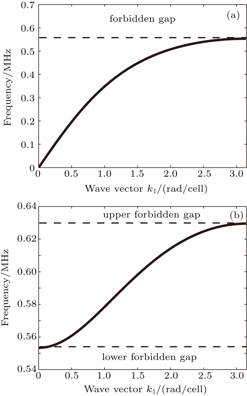
The corresponding linear dispersion law describing small amplitude waves of the form A0exp(i(k1n + k2m − ωt)) is given by
This dispersion relation shows that our network is a band-pass filter with the cutoff frequency . For values of ki chosen in the Brillouin zone (0 < ki < π) with i = 1,2, we present the evolution of the angular frequency for the n direction and for two specific values of transversal wave numbers k2 in Fig. 2.
Fig. 2. The linear dispersion of the network according of the wave vector k1 (rad/cell) for u01 = 2.5786 × 10⁶ rad/s, u02 = 2.5786 × 10⁶ rad/s, Cr1 = 0.3, and Cr2 = 0.3 : (a) k2 = 0 and (b) k2 = π.
The discreteness and nonlinearity of these coupled ODEs render their exact analytical investigation obviously intractable. To manage this difficulty, we can use the continuum approximation by setting Vn,m(t) → V(n,m,t). We suppose that the spacing between two adjacent sections is the same in the two directions (h1 = h2 = h). To express the space variables n and m in units of cell, the lattice spacing h is taken as equal to one. Then, using this approximation, we obtain from Eq. (2) the following two-dimensional partial differential equation (PDE) for the perturbed voltage V:
To find the traveling wave solutions of this equation we introduce the Gardner-Morikawa transformation of the independent variables. This specific transformation is widely used for the analytical investigation of nonlinear discrete lattices[25,39,75,76] owing to its feature of properly balancing the nonlinearity and dispersion after expansion. For our two-dimensional network, it reads
where ϵ ≪ 1 is a formal parameter while x and y are the instantaneous coordinates of the moving structure in the network. Correspondingly, υ1 and υ2 are the components of the displacement velocity in these respective directions. The use of these variables also implies that the time and space derivative operators are transformed according to
By inserting Eqs. (5)–(8) into Eq. (4) and collecting terms of the same order in ϵ, we find that the coefficient proportional to lowest order (ϵ2) gives
In the next order, after integration and setting the constant of integration to zero, we obtain
The solutions of Eq. (2) can be obtained by solving Eqs. (9) and (10). To this end, we define the single variable
where υc is the front wave velocity and θ is the propagation direction of the wave relative to the x-direction. By considering this definition, equation (9) becomes the following ordinary differential equation:
This last equation is identically verified if we express υ1 and υ2 in terms of θ according to
with
Inserting Eqs. (11) and (13) into Eq. (10), then integrating and setting the constant of integration to zero lead to
where Cr = Cr1 cos2(θ)+Cr2 sin2(θ).
3. Dynamical studies and sine-Gordon expansion-method
3.1. Dynamical studies
Now, we turn our attention to the dynamical studies of the above characteristic ODE of the network. Various solutions of this equation can be obtained depending on the value of the parameter υc. When Cr (υ0 + 2ϵυc) ≠ 0, equation (14) can be reduced to a two-dimensional dynamical system
System (15) has a first integral defined as
where K is an integral constant and U(ψ) is an effective potential defined by
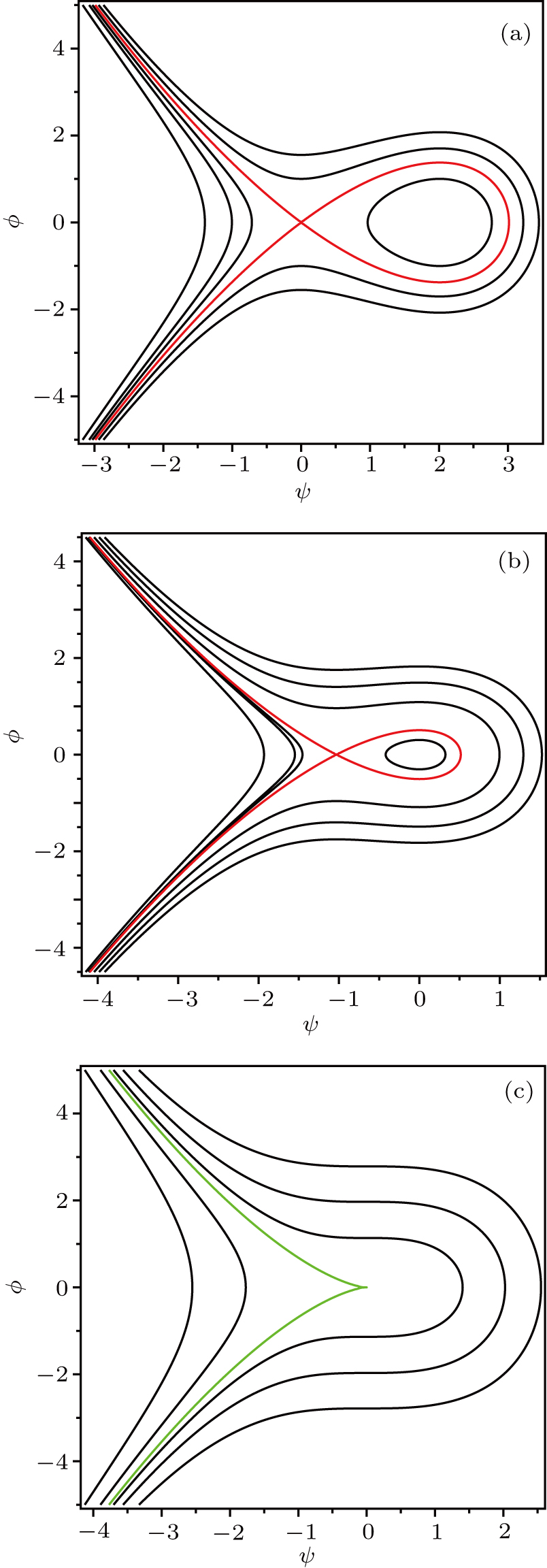
We observe that system (15) has several singular points depending on the value of the front wave velocity υc. In fact, O(0, 0) is always the equilibrium point of system (15) independently of the value and sign of this parameter. Equation (15) has one additional equilibrium point . When υc > 0 or , A1 is a center and O(0,0) is a saddle point. For , the natures of these equilibrium points change: O(0,0) becomes a center and A1 is a saddle point. This analysis is confirmed by the phase plane plot of the system sketched in Fig. 3.
Fig. 3. (color online) The phase portraits of system (15) in the (ψ, ψ′)-phase plane for u01 = u02 = 2.5786 × 10⁶ rad/s, Cr1 = Cr2 = 0.3, θ = π/32, α = 0.21 V−1, β = 0: {(a)} υc > 0 or υc < −υ0/2ϵ, (b) −υ0/2ϵ < υc < 0, (c) υc = 0.
On the preceding figure (Fig. 3), we distinguish the following types of orbits: (i) a homoclinic orbit (red curve) which corresponds to a pulse soliton or bright solitary waves (BSW) solution of Eq. (10); (ii) periodic orbits (closed black curve) which correspond to periodic traveling wave solutions of equation (10). From these figures, we summarize crucial conclusions as follows. (i) If υc ≠ 0, system (15) always has an homoclinic orbit which is asymptotic to the saddle and encloses the center. In this case, there also exists a family of periodic orbits which enclose the center and fill up the interior of the homoclinic orbit. (ii) When υc = 0, the equilibrium point O(0,0) is a cusp.
3.2. The sine-Gordon expansion-method
In this subsection, we present the sine-Gordon expansion method which will later be utilized to investigate the solitary waves of the coupled electric transmission line. This method is based on the sine-Gordon equation and a traveling wave transformation.[64–66]
In fact, consider a nonlinear partial differential equation (NLPDE) with two independent variables x and t
In general, the left hand side of Eq. (18) is a polynomial in U and its various derivatives. Assuming that U(x, t) = U(ξ), ξ = k1x − υct, where k1 and υc are constants to be determined later, then equation (18) is reduced to an ordinary differential equation
where G is a polynomial of U and its various derivatives.
We consider that the sought solution can be expressed as follows:
According to Refs. 68–70, equation (20) can be rewritten as
where the function w(ξ) = U(ξ)/2 satisfies the following relation:
Equation (22) is variables separable, and we obtain the following two significant equations upon solving it:
The parameter Im is, in most cases, a positive integer that can be determined by considering the homogeneous balance between the highest order derivative and the highest order nonlinear terms appearing in ODE (19). Collecting and setting the coefficients of terms of the form sini(w)cosj(w) to zero yield a system of coupled nonlinear algebraic equations. Solving this system using Maple gives the values of ai, bi, a0, k1, and υc. Finally, upon substituting these values in Eq. (20), we obtain the traveling wave solutions to Eq. (19).
4. Exact solution of Eq. (14)
4.1. Implementation of the sine-Gorgon method
Now we focus our attention on the derivation of the bright solution of the two-dimensional partial differential equation (4). To this end, we introduce the variable ξ = μz and equation (14) becomes
in which
On balancing the nonlinear term ψ2 and the highest order derivative term ψ″ in Eq. (25), we find that Im = 2. So, we may express the solutions of this equation in the form
Substituting Eqs. (27) and (28) in into Eq. (26), and equating the coefficients of each power of sini(w)cosj(w) to zero, we obtain a system of algebraic equations of the parameters a0, a1, a2, b1, b2, and μ, i.e.,
It appears that there are three more equations than the six variables sought for. Such a large number of coupled nonlinear algebraic equations can be obviously very challenging for human manipulation. On the contrary, computer algebra tools such as Maple, Mathematica, or MuPAD are very powerful for such tasks, especially as these equations are all polynomial. For the explicit solutions that are of interest to us in this paper, and disregarding the trivial (constant) solutions, we find with the help of Maple that they depend on the combination of the physical parameters as considered below.
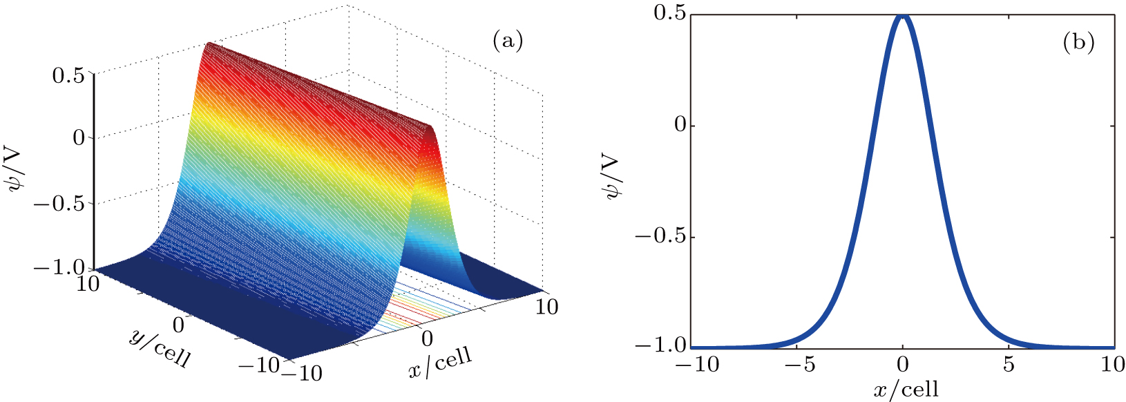
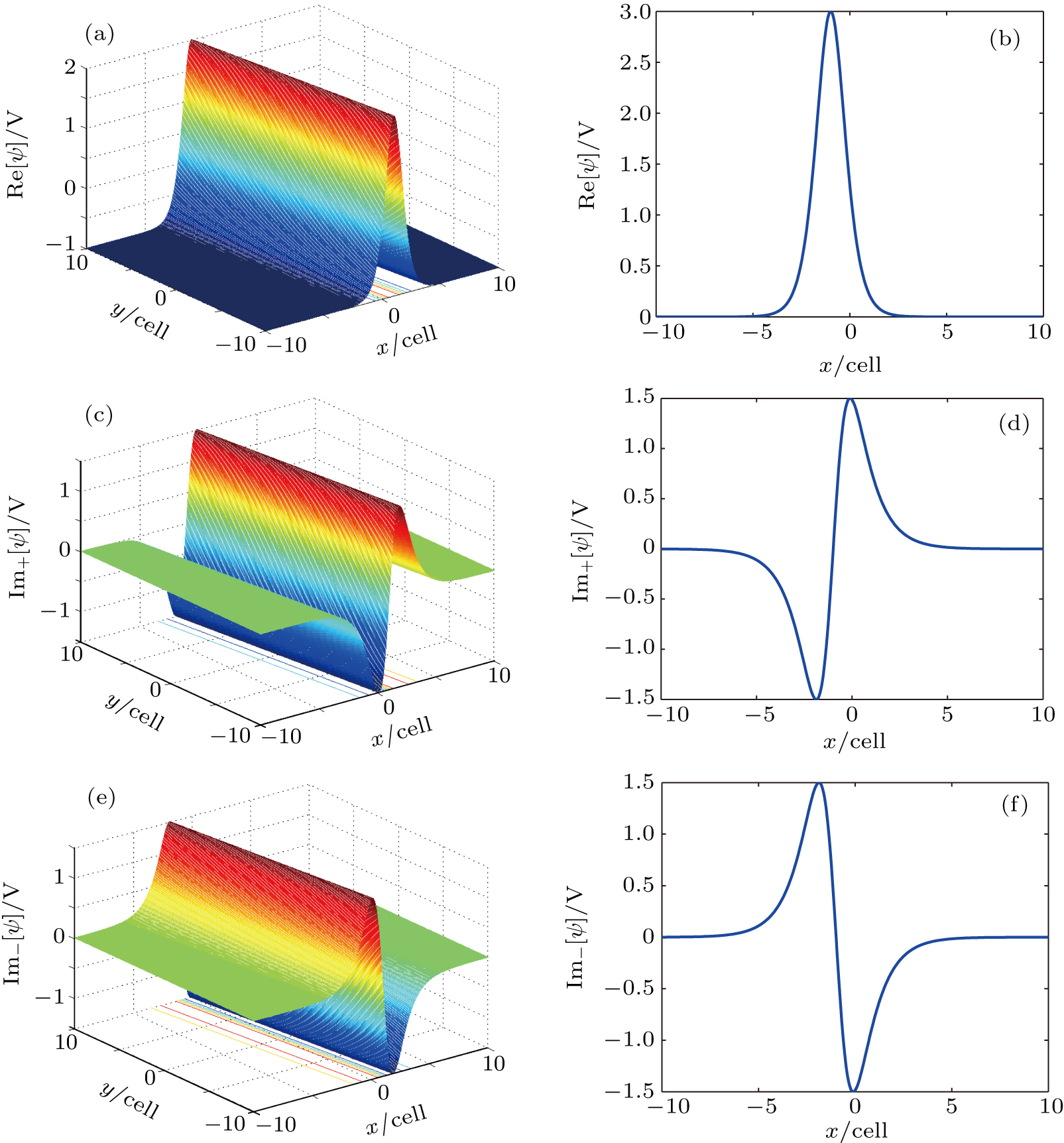
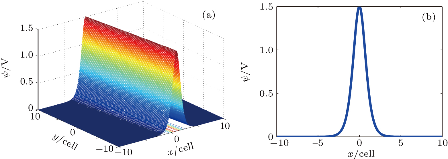
Fig. 6. (color online) The 3D and 2D bright and breathers solutions of Eq. (35) for A = 1, B = 1, θ = π/32, t = 0, −10 < x < 10: (a), (c), (e) −10 < y < 10; (b), (d), (f) y = 10.
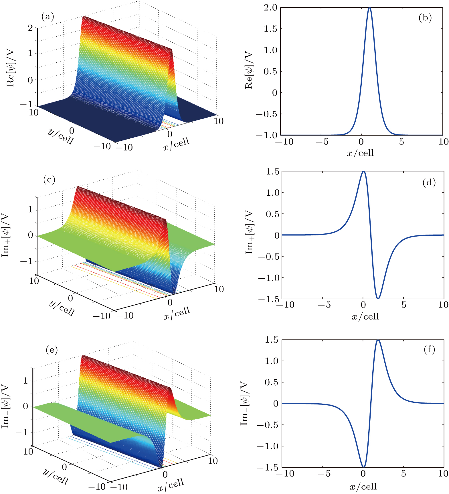
Fig. 7. (color online) The 3D and 2D bright and breathers solutions of Eq. (31) for A = −1, B = 1, θ = π/32, t = 0, −10 < x < 10: (a), (c), (e) −10 < y < 10; (b), (d), (f) y = 10.
4.2. Supplementary solutions
This subsection is devoted to the computation of other exact solutions of Eq. (14) which correspond to bounded traveling wave solutions of Eq. (1). Equation (16) can be written in the form
Let
If Δ < 0, f(ϕ) admits three real roots ψ1, ψ2, and ψ3 with ψ1 ≥ ψ2 ≥ ψ3. In this case, we have
From Eq. (41), we obtain
By using the first equation (38), one obtains
The exact solutions of Eq. (14) are obtained from the results of Eq. (43). Some transformations[77] lead to
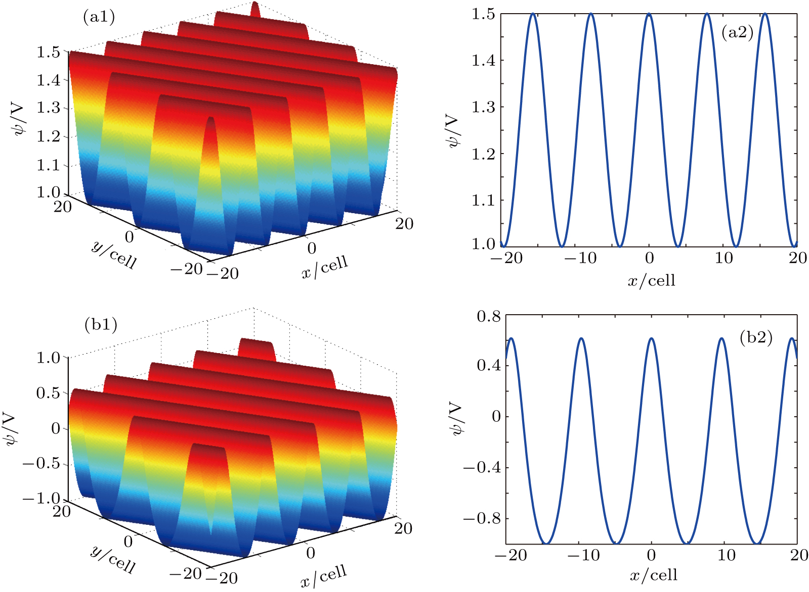
The last equation of Eq. (42) clearly shows that these roots do not all have the same sign. Thus, we have the following two situations: (i) ψ1 > 0, ψ2 > 0, ψ3 < 0; and (ii) ψ1 > 0, ψ2 < 0, ψ3 < 0. The graphs of Eq. (44) for these two situations are shown in Figs. 8(a) and 8(b), respectively, which are the periodic wave solutions of Eq. (14).
Fig. 8. (color online) The 3D and 2D periodic solutions of Eq. (44) for B = 0.7, θ = π/6, t = 0, −20 < x < 20: (a1), (b1) −20 < y < 20; (a2), (b2) y = 0. (a) ψ3 = −0.6, ψ2 = 1, and ψ1 = 1.5. (b) ψ3 = −1.6, ψ3 = −1, and ψ1 = 0.6154.
We remark that, for ψ2 = ψ3 = 0 and K = 0, we have and solution (44) is identical to the bell profile solitary wave solution (31). Similarly, for and , we have , and solution (44) is identical to the bell profile solitary wave solution (33).
5. Physically exploitable solutions in the particular case of the electrical network
The results obtained in this paper are bright soliton, grey soliton, breathers, and periodic solutions. These solutions are used for the information transmission through the electrical lattice and can also help to explain the dynamics of many other discrete lattices like a chain of atoms. Particulary, for the case of the two-dimensional nonlinear electrical network in Fig. 1, we have the following exploitable results.
5.1. Situation 1: υc > 0 or υc < −υ0/2ϵ (A > 0 and B > 0)
In this case, both bell-shaped soliton as well as periodic solitary waves can be propagated in the network. For K = 0, the explicit expression of voltage corresponding to the pulse-like signal is given by
with and ; ϵ0 and Cr are defined by Eqs. (13) and (14), respectively. This expression involves four main quantities, including the amplitude V0, the speed υp1, the reduced propagation direction θ, and the width Ls = 1/μ0. From the expression of υp1, it appears that the soliton can effectively exist for ; and that of μ0 shows clearly that the width originates from the quadratic nonlinearity and crucially depends on the signal’s amplitude V0. It is also worth to notice that the envelope velocity of the pulse is dependent on the amplitude V0 of the signal. For positive front wave velocity υc, the envelope velocity increases with the amplitude V0 and decrease in the contrary case. Thus, since the wave velocity is amplitude dependent, two adjacent pulse solitons of different amplitudes will interact in the network because they propagate at different speeds.
When , the explicit expression of voltage corresponding to the periodic signal voltage is given by
in which
5.2. Situation 2: −υ0/2ϵ < υc < 0 (A < 0 and B > 0)
Here, the types of waves supported by the network are periodic and grey solitary waves. The former exists for and is also described by Eq. (46). The grey soliton signal voltage is obtained for , and reads
with and υ0 and Cr defined by Eqs. (13) and (14), respectively. It is also described by the same four parameters as in the case of bright soliton of the preceding situations.
6. Conclusion
We have investigated the transverse wave solutions in a system of coupled nonlinear partial differential equations that was earlier shown to govern the dynamics of waves in a coupled nonlinear inductor-capacitor network. Firstly, using the dynamical studies we found that the phase portrait of the system admits an homoclinic orbit and periodic orbits which respectively correspond to a bright soliton and periodic wave solutions of the equation governing the network. Next, via the sine-Gordon expansion-method and direct integration, we obtained all traveling wave solutions of these coupled equations such as complex, elliptic, and hyperbolic function solutions. The two- and three-dimensional graphics of all obtained solutions in this work are given. Finally, some of these solutions that are physically exploitable in the particular case of the network considered (Fig. 1) are presented. These solutions are used for the information transmission through the electrical lattice and can also help to explain the dynamics of many other physical systems. The sine-Gordon expansion-method used here is powerful and can be also applied to other nonlinear equations in mathematical physics.


