In the last few years, with the development of the economy, the influence of traffic jams on people’s life has become more and more serious. Therefore, many traffic flow models^[1–15] have been proposed to research traffic congestion by using linear analysis and nonlinear analysis, such as the car-following models,^[16–28] the cellular automation models,^[29–32] the gas kinetic models,^[33–36] and the hydrodynamic lattice models.^[37–40]

The research of transport has been gradually developed into three major directions. Generally, traffic flow models have been divided into three types: macroscopic models, microscopic models, and mesoscopic models. One of the most typical models is the optimal velocity model (for short, OVM) proposed by Bando et al.^[41] in 1995, in which the differential equation of the optimal velocity model is obtained by Taylor expansion. The problem of infinite acceleration is solved in OVM: it can simulate many qualitative characteristics of the actual traffic flow, such as traffic congestion, congestion evolution, and so on. In order to solve the problems of high acceleration and unrealistic deceleration in OVM, Helbing and Tilch^[42] developed a generalized force model (for short, GFM) by considering the negative velocity difference on the basis of OVM. But GFM cannot describe the delay time of car motion and the kinematic wave speed at jam density. Jiang et al.^[43] put forward the full velocity difference model (for short, FVDM) by considering the positive velocity difference based on GFM. However, FVDM has too high deceleration. Ge et al.^[44] put forward a two-velocity difference model (for short, TVDM) to solve these problems. There is no doubt that the authors have prominently contributed to the modeling of traffic flow and to promoting the development of the theory for traffic flow. Previous research results have enriched and improved the model of traffic theory.

As is well known, roads are not always straight and there are lots of curved roads;^[45,46] however, there has been little research on curved roads using the car-following model. Therefore, based on FVDM, this paper studies the evolution trend of the traffic flow in a bend. We will present a modified model for the curved road and investigate the stability from the perspective of energy consumption.^[47]

On the basis of previous studies, a new car-following model is proposed. In section 2, based on FVDM, the new model including the influence of the friction coefficient and radius is put forward. Moreover, the control analysis method will be used to analyze the improved model. In section 3, the new model is analyzed by the nonlinear analysis near the critical point, then the time-dependent Ginzburg–Landau (TDGL) equation and its corresponding solution are derived. In section 4, the modified Korteweg–de Vries (mKdV) equation is given. In section 5, numerical simulations are present. The conclusions are given in section 6.

We consider the case in which vehicles run ahead on a single-lane curved road under open boundary conditions. At the same time, the effects of the friction coefficient and curve radius are also considered. A centripetal force acts on the running vehicles, where μ is the coefficient of the friction, m is the mass of the vehicle, and g is the acceleration due to gravity. The length of the curve is , where θ is the radian and r is the radius.

According to the above mentioned idea, we derive a new mathematical model. The motion equation is 1 where is the position of the vehicle at time t, a is the sensitivity which corresponds to the inverse of the delay time, and λ is a parameter of FVDM. With the relationship between the radian and radius of the curved road section 2 equation (1) can be rewritten as 3

The optimal velocity function is proposed as follows: 4 where is the maximum angular velocity and is the safe arc length of the vehicle. The other parameters are the same as before. The relationship between the maximum angular velocity and the friction coefficient is 5 The theoretical values of the real traffic situation are higher than the maximum angular velocity, then we adopt a constant coefficient α. So the optimal velocity function is rewritten as 6

In addition, we take into account the relationship between the energy consumption and vehicle stability. The energy consumption of each vehicle on a curved road can be investigated in more details on the basis of the kinetic energy theorem, which describes every vehicle to do work through consuming energy. By describing the change of the vehicle in two adjacent moments, the change of the kinetic energy is defined as 7 where and are the velocities of vehicle i in the two successive time steps.

Then linear stability analysis can be conducted. We can compare the new model for traffic flow on a curved road with the previous models. The derivative of the radian is the angular velocity. Therefore, the stable condition can be given as follows: 8 where and . We assume that the leading vehicle is not effected by others and runs on the curved road with a constant speed , then the steady state is as follows: 9

The linearized system (8) can be calculated and the steady state space equation is 10 where , , , derivatives

By Laplace transformation, the linearized system can be written as 11 where , L denotes the Laplace transform. The characteristic polynomial is , where s is a complex variable. Then we can obtain 12

As is in positive correlation with , so we have 0. We also have 0, then the condition for is stable. We consider , which is the same as 13 we can obtain the sufficient condition by the above analysis, which can be rewritten as 14

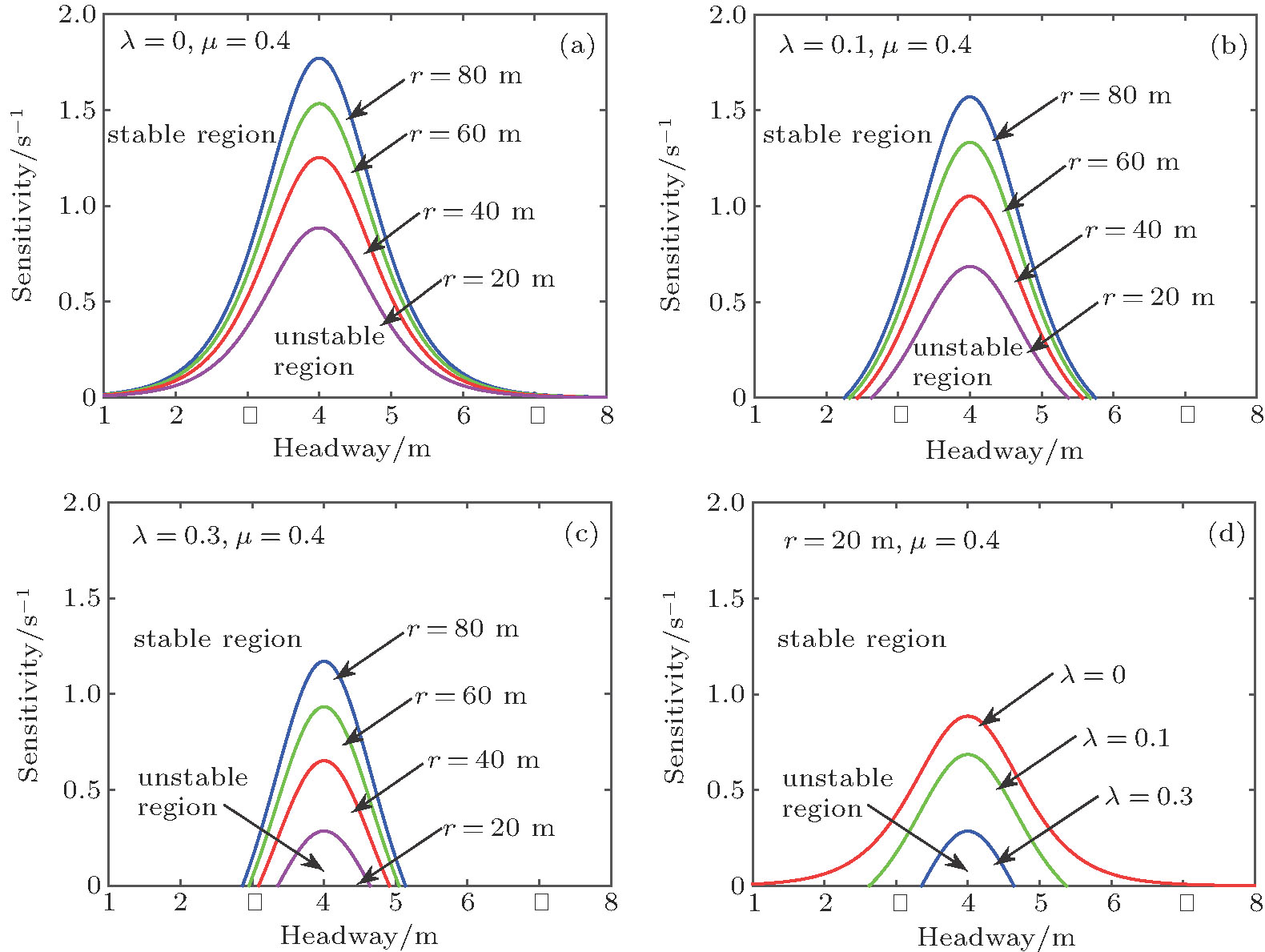
For small disturbance with long wavelengths, the uniform traffic flow is instable in the condition 15 In summary, we obtain the stability condition of the traffic flow as follows: 16

Figure 1 shows the phase diagram in the ( , ) plane, where is the headway and is the sensitivity which corresponds to the inverse of the delay time. The solid lines show the neutral stability curves with different λ. It shows the unstable region, and the critical points decline with decreasing parameter r.

Fig. 1.

	Figure Option ViewDownloadNew Window
	Fig. 1. (color online) The phase diagram of the model with different parameters λ and r.

As can be seen from Figs. 1(a)–1(c), when g and μ are unchanged, with the decrease of r (r = 80 m, 60 m, 40 m, 20 m) and the increase of λ (λ = 0, 0.1, 0.3), the unstable region gradually becomes smaller, and the stable region gradually becomes larger. Then the traffic flow is more stable. Especially, from Fig. 1(d), the stable region reaches the largest when the values are selected as λ = 0.3, μ = 0.4, and r = 20 m.

Figure 2 shows the phase diagram in the ( , ) plane, where is the headway and is the sensitivity which corresponds to the inverse of the delay time. The solid lines show the neutral stability curves with different λ. It shows the unstable region, and the critical points decline with decreasing parameter μ.

Fig. 2.

	Figure Option ViewDownloadNew Window
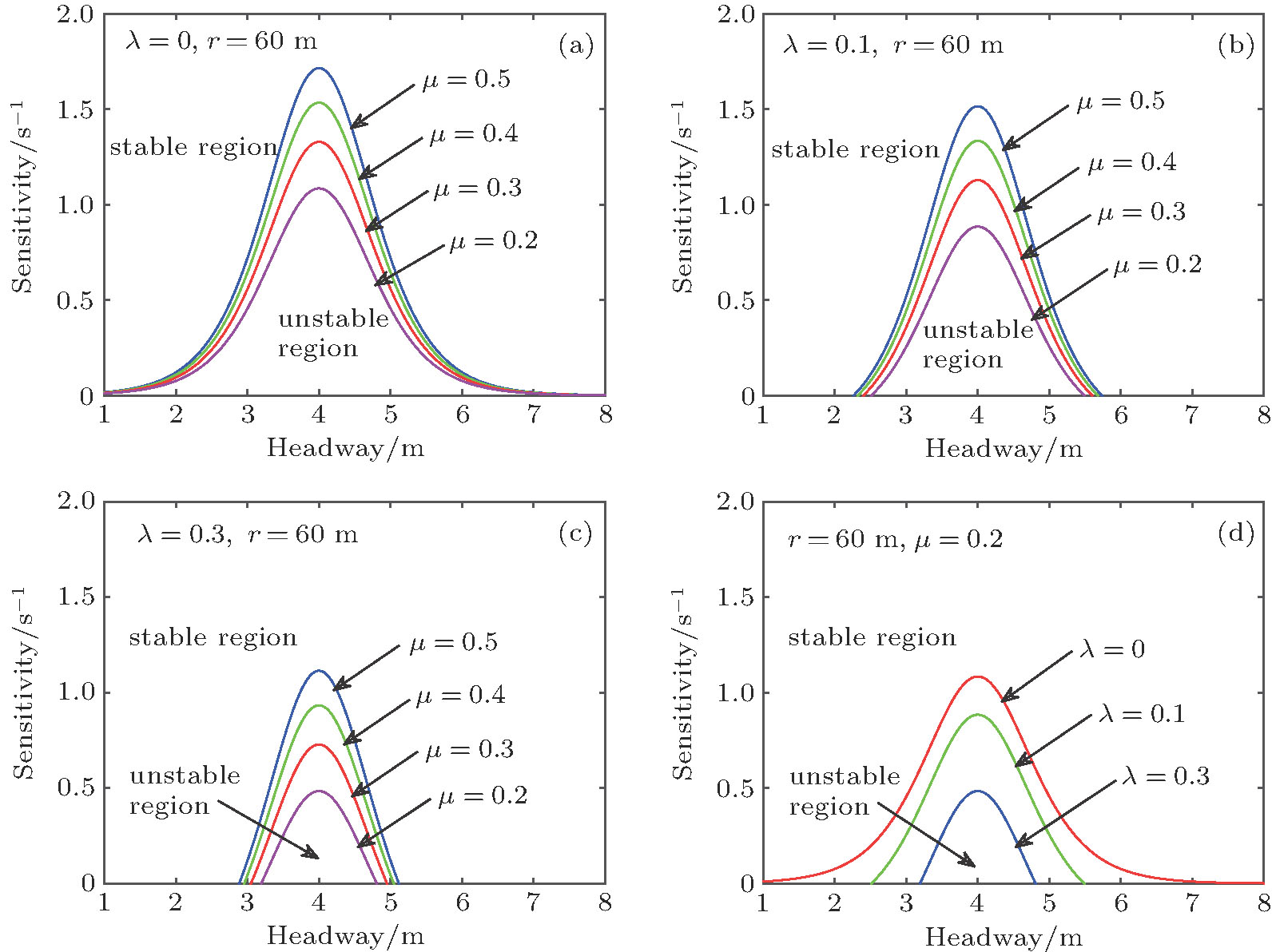
	Fig. 2. (color online) The phase diagram of the model with different parameters λ and μ.

As we can see from Fig. 2(a)–2(c), when g and r are fixed, with the decrease of μ (μ = 0.5, 0.4, 0.3, 0.2) and the increase of λ (λ = 0, 0.1, 0.3), the unstable region gradually becomes smaller, the stable region gradually becomes larger. Then the traffic flow is more stable. Especially, from Fig. 2(d), the stable region reaches the largest when the values are selected as λ = 0.3, μ = 0.2, and r = 60 m.

In the car-following models, the nonlinear density wave equation is derived to describe the propagation characteristics of traffic congestion. In this part, we adopt the method of nonlinear analysis to investigate the problem. On the coarse grain scale, we describe the traffic flow by using the long wavelength models and then obtain the solution of the equation. The slow changing behavior of long waves near the critical point is analyzed. We assume that τ is very small, then equation (3) can be rewritten as follows: 17 Furthermore, equation (17) can be rewritten as follows: 18 The slow scales for space variable i and time variable t are introduced, and the slow variables and T are defined as follows: 19 The headway is set as 20 By bringing Eqs. (20) and (21) into Eq. (19), and expanding to the fifth-order of ε, we obtain 21 where the coefficients m_j are given in table 1.

Table 1.

Table 1.

Table 1. The coefficients mj of the model. . m1 m2 m3 m4 m5 m6 m7

Table 1. The coefficients mj of the model. .

Now, we consider the traffic flow near critical point . Through taking , the second- and third-order terms of ε are eliminated from Eq. (22), which leads to the simplified equation 22 By transforming and T into variables and , and taking , equation (22) is rewritten as follows: 23 By adding term on both left and right sides of Eq. (23) and performing and , we obtain 24

We define the thermodynamic potentials 25 By rewriting Eq. (25) with Eq. (26), the TDGL equation is derived as 26 27 where indicates the function derivative. The TDGL (27) has two steady-state solutions except trivial solution S = 0. One is the uniform solution 28 The other is the kink solution 29 where x₀ is a constant. Equation (30) represents the coexisting phase. By the condition30 we obtain the coexisting curve from Eq. (26) in terms of the original parameters 31 The spinodal line is given by the condition 32 From Eq. (26), we obtain the spinodal line described by the following equation: 33 The critical point is given by the condition and Eq. (33), 34

Similarly, from the derivation of the TDGL equation, we study the slowly varying behavior at long wavelengths near the critical point. We abstract the slow scale for space variable i and time variable t. By inserting and into Eq. (13), one obtains 35 where the coefficients j_i are given in table 2.

Table 2.

Table 2.

Table 2. The coefficients ji of the model. . j1 j2 j3 j4 j5

Table 2. The coefficients ji of the model. .

In the table, and . In order to derive the regularized equation, we make the following transformation: 36 then the standard mKdV equation with an correction term is obtained as follows: 37

If we ignore the , they are just the mKdV equations with a kink solution as the desired solution 38 Then, assuming that , we take into account the correction. For the purpose of determining the selected value of the velocity c for the kink solution, it is essential to satisfy the solvability condition. As where we obtain the general velocity c, 39 Therefore, the general kink–antikink soliton solution of the headway from the mKdV equation is obtained as 40 where . This kink soliton solution also represents the coexisting phase, and the kink solution (41) agrees with the solution (30) obtained from the TDGL equation. Therefore, the jamming transition can be described by both the TDGL equation with a nontravelling solution and the mKdV equation with a propagating solution.

In this section, the numerical simulation is carried out for theoretical analysis through the computer. With the periodic boundary condition, the initial conditions are given as follows: for , , for , for j = 51. We choose the total number of cars and the sensitivity as N = 100 and a = 1.6.

Figure 3 shows the space–time evolution of the headway after time steps with the fixed parameters λ, μ, g and the varied parameter r. A series of simulations are carried out under the periodic conditions for the new car-following model with different parameters. It can exhibit the kink–antikink solutions propagating backwards. Especially, when r is the minimum, the traffic flow model becomes the most stable. From Fig. 3(a) with λ = 0.3, μ = 0.4, g = 9.8 m/s², r = 70 m, it is clear that the traffic flow is very unstable and chaotic on a curved road. When a small disturbance is added into the uniform traffic flow, the propagating backward stop-and-go traffic jam appears, which is very similar to the mKdV solution. From Fig. 3(a) to Fig. 3(b), the traffic flow model congestion situation has a small improvement. Gradually, in Figs. 3(c) and 3(d) with r = 50 m and r = 40 m, respectively, it can be seen that the traffic flow model of congestion on a curved road has been significantly improved. It is very stable. It is obvious that the amplitude of the kink–antikink soliton weakens gradually with increasing parameter λ and decreasing parameter r.

Fig. 3.

	Figure Option ViewDownloadNew Window
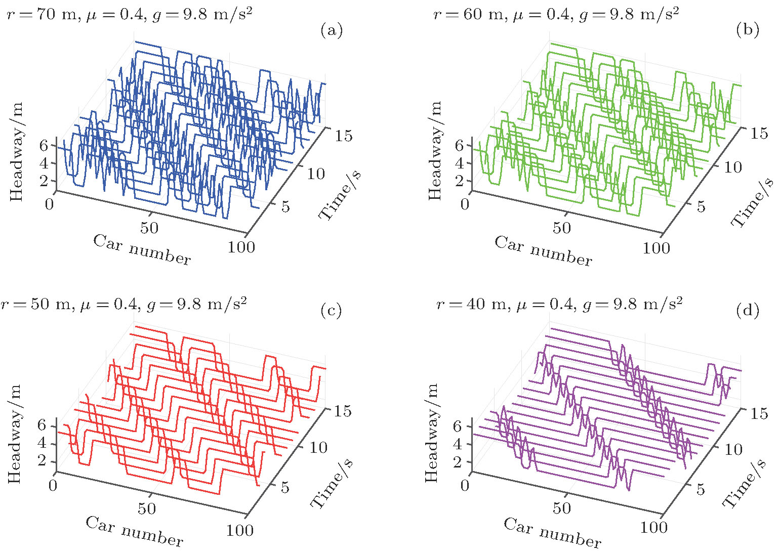
	Fig. 3. (color online) Space–time evolution of the headway after t = 10000 with different r.

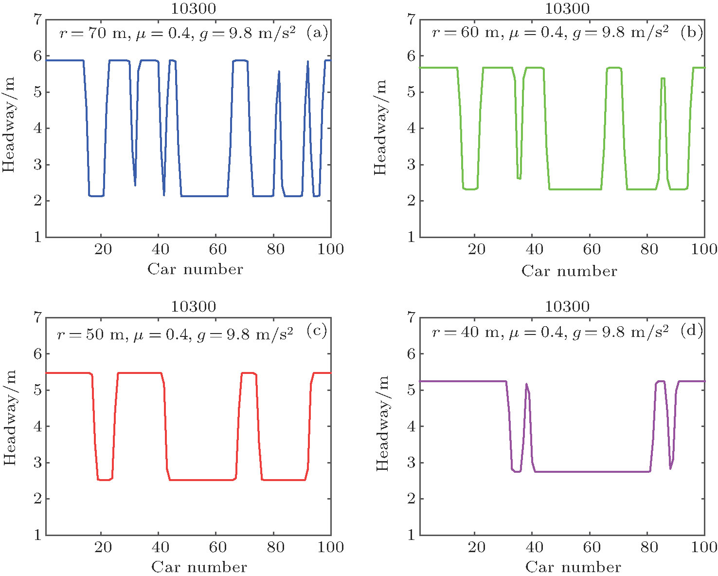
Figure 4 shows the headway profiles and density waves for different friction coefficients and radii of curvature at t = 10300 corresponding to the panels in Fig. 3; similar results are obtained from Fig. 3. Figures 4(a)–4(d) correspond to radii of curvature r = 70 m, 60 m, 50 m, 40 m, respectively. The other parameters are unchanged. As the radius gradually becomes smaller, the traffic flow model becomes more stable. The numerical simulation and theoretical analysis are consistent.

Fig. 4.

	Figure Option ViewDownloadNew Window
	Fig. 4. (color online) Headway profiles of the density wave at t =10300 corresponding to Fig. 3.

Figure 5 exhibits the space–time evolution of the headway after time steps with the fixed parameter λ, g, r and the varied parameter μ. A battery of simulations are carried out under the periodic conditions for the new car-following model on a cured road with different parameters. It shows the kink–antikink solutions propagating backwards. It can be seen that the traffic flow becomes more stable with increasing parameter μ. From Fig. 5(a) with λ = 0.3, r = 60 m, g = 9.8 m/s², μ = 0.5, it is clear that the traffic flow is very unstable and chaotic on a curved road. When a small disturbance is added into the uniform traffic flow, the propagating backward stop-and-go traffic jam appears, which is very similar to the mKdV solution. From Fig. 5(a) to Fig. 5(d), μ decreases while the other parameters are not changed. It can be seen from the graph that the traffic flow model of congestion on a curved road has been significantly improved. It is obvious that the amplitude of the kink–antikink soliton weakens gradually with increasing parameter λ and decreasing parameter μ. In general, the smaller the parameter μ, the more stable the traffic flow.

Fig. 5.

	Figure Option ViewDownloadNew Window
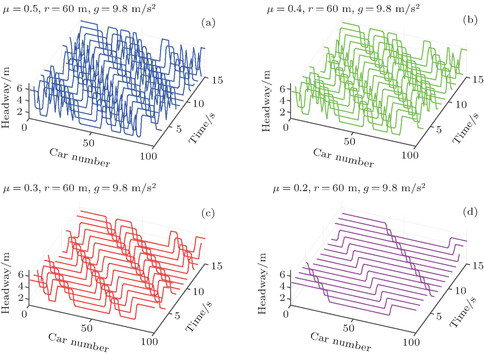
	Fig. 5. (color online) Space–time evolution of the headway after t = 10000 with different μ.

Figure 6 exhibits the headway profiles and density waves for different μ and r at t = 10300 corresponding to the panels in Fig. 5. From Fig. 5, similar results are obtained. From Fig. 6(a) to Fig. 6(d), the friction coefficient changes from 0.5 to 0.2, with λ = 0.3, g = 9.8 m/s², r = 60 m. From the figure, we find that the traffic flow on the curved road is more stable with the small coefficient of friction.

Fig. 6.

	Figure Option ViewDownloadNew Window
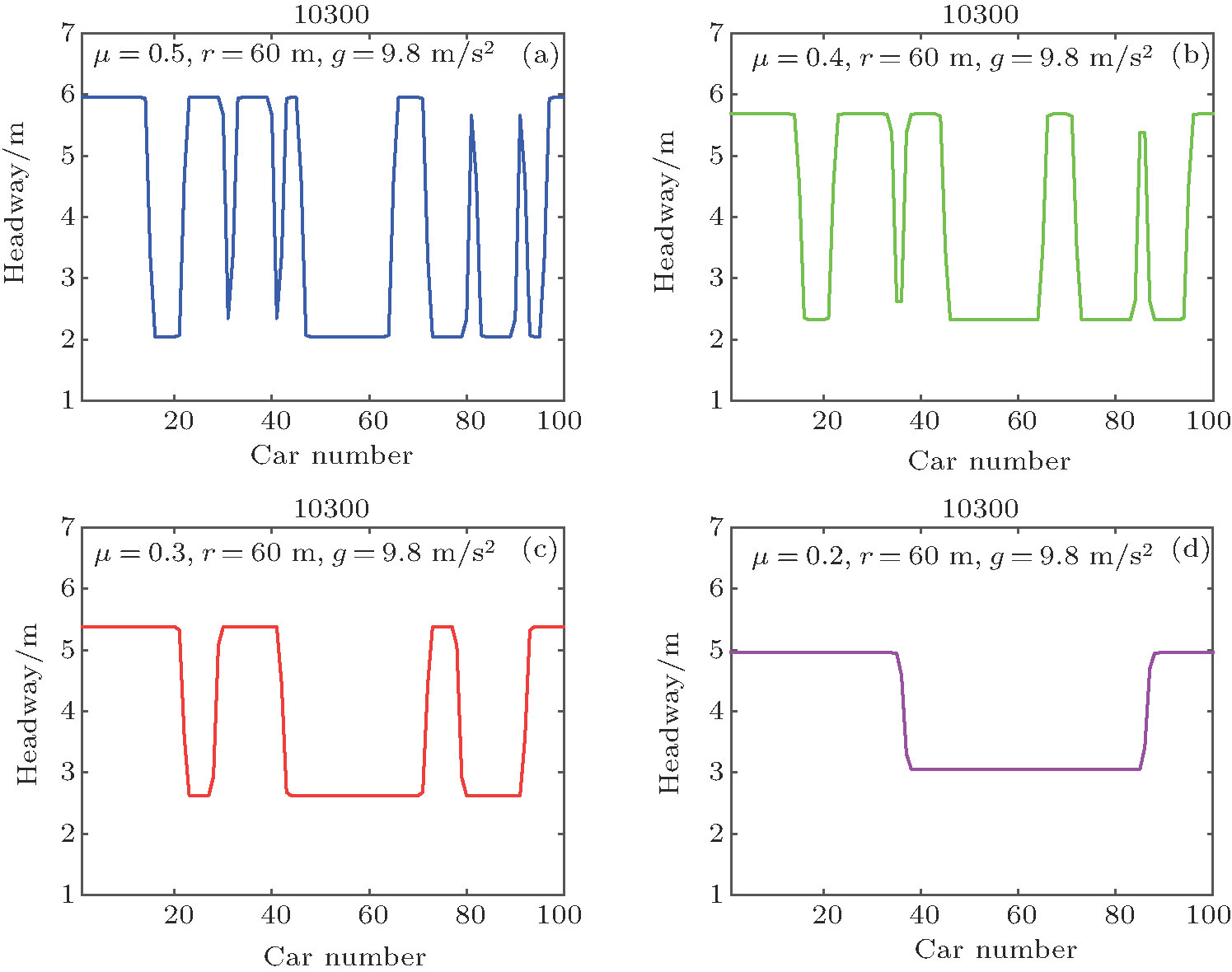
	Fig. 6. (color online) Headway profiles of the density wave at t =10300 corresponding to Fig. 5.

The stability of the vehicle can be reflected in many aspects; now we analyze from the perspective of energy consumption. We study the relation between the energy consumption and the stability. The change of energy consumption of a vehicle running on a curve depends on parameter λ.

Figure 7 shows the distribution of energy consumption for the models with different λ. The blue curve denotes the model with λ = 0, the numerical simulation result is consistent with that in OVM proposed by Bando et al. The area of loop in OVM is the largest, so it is most unstable. The green curve denotes the model with λ = 0.1 and the red curve denotes the model with λ = 0.3.

Fig. 7.

	Figure Option ViewDownloadNew Window
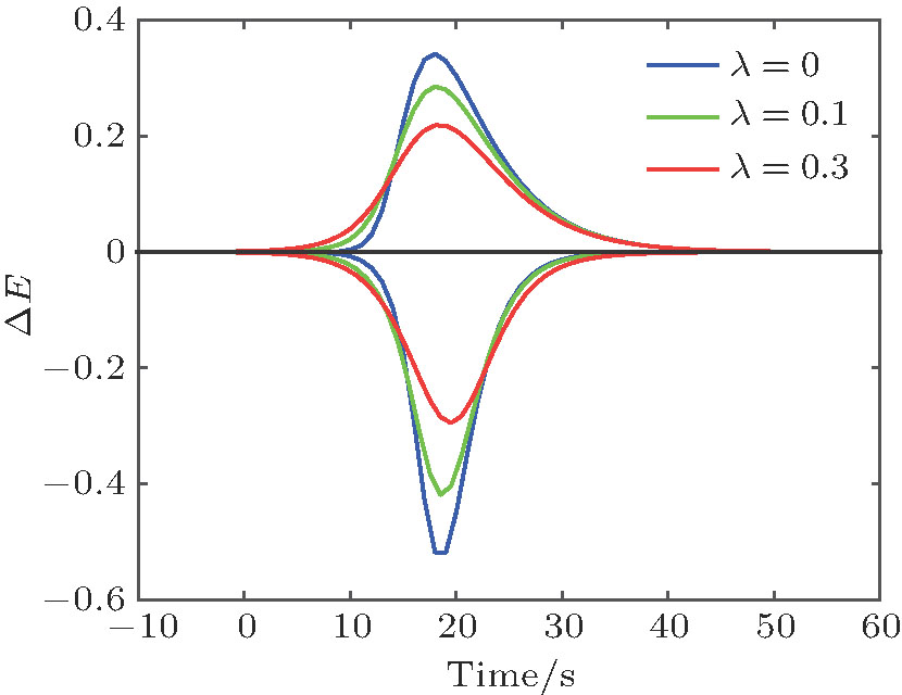
	Fig. 7. (color online) Profile of energy consumption of vehicle with different parameter λ.

From Fig. 7, we can see two regions with and . denotes the energy dissipation in the deceleration process of a vehicle and describes the energy dissipation of a vehicle during acceleration. It can be seen clearly in Fig. 7 that the areas of the acceleration process and the deceleration process are not symmetrical. The area of the deceleration process is larger than that of the acceleration process. This shows that the energy consumption of the deceleration process is greater. In a word, the energy consumption has decreased with the increase of λ.

The curved road is very common, so it is important to study the curved road traffic flow. The vehicle on a curved road is affected by many factors. In our model, by means of linear analysis and nonlinear analysis, we study the evolution trend of the traffic flow in a bend and analyze the influence of the friction coefficient and the radius of the curve on the traffic. We also analyze stability from the perspective of energy consumption. The neutral stability line and the critical point are obtained by the linear stability analysis. The TDGL equation has been derived to describe the traffic behavior near the critical point by applying the reductive perturbation method. In addition, the mKdV equation has been derived and we show the relationship between the TDGL and the mKdV equations. Finally, the analytical results are found to be in good agreement with the numerical simulation.