Different angle-resolved polarization configurations of Raman spectroscopy: A case on the basal and edge plane of two-dimensional materials
Liu Xue-Lu1, 2, Zhang Xin1, 2, Lin Miao-Ling1, 2, Tan Ping-Heng1, 2, †
State Key Laboratory for Superlattices and Microstructures, Institute of Semiconductors, Chinese Academy of Sciences, Beijing 100083, China
College of Materials Science and Opto-Electronic Technology, University of Chinese Academy of Sciences, Beijing 101408, China


† Corresponding author. E-mail: phtan@semi.ac.cn

Abstract

Angle-resolved polarized Raman (ARPR) spectroscopy can be utilized to assign the Raman modes based on crystal symmetry and Raman selection rules and also to characterize the crystallographic orientation of anisotropic materials. However, polarized Raman measurements can be implemented by several different configurations and thus lead to different results. In this work, we systematically analyze three typical polarization configurations: 1) to change the polarization of the incident laser, 2) to rotate the sample, and 3) to set a half-wave plate in the common optical path of incident laser and scattered Raman signal to simultaneously vary their polarization directions. We provide a general approach of polarization analysis on the Raman intensity under the three polarization configurations and demonstrate that the latter two cases are equivalent to each other. Because the basal plane of highly ordered pyrolytic graphite (HOPG) exhibits isotropic feature and its edge plane is highly anisotropic, HOPG can be treated as a modelling system to study ARPR spectroscopy of two-dimensional materials on their basal and edge planes. Therefore, we verify the ARPR behaviors of HOPG on its basal and edge planes at three different polarization configurations. The orientation direction of HOPG edge plane can be accurately determined by the angle-resolved polarization-dependent G mode intensity without rotating sample, which shows potential application for orientation determination of other anisotropic and vertically standing two-dimensional materials and other materials.

1. Introduction

Raman spectroscopy is a fast and non-destructive characterization technique, which has been widely used to characterize kinds of two-dimensional materials (2DMs),[1] such as graphene, transition metal dichalcogenides (TMDCs), and recently-revealed anisotropic black phosphorus (BP), , and . It can afford information on the layer thickness,[2] stacking order,[35] surface adsorbates,[6] the strength of interlayer interactions[7,8] etc. Angle-resolved polarized Raman (ARPR) spectroscopy is an important branch of Raman spectroscopy. The typical polarization configuration is that the polarization directions of both incident and out scattering lights are fixed along the main axis (x, y, z). Under the back scattering condition, one can use two letters (HV, VH, VV or HH) to separately denote the polarization directions of both incident and out scattering lights. Angle-resolved polarized Raman spectroscopy has been used to resolve and assign Raman peaks[1,810] and characterize the aligned orientation of single-wall nanotubes,[11] and bundled multi-wall nanotubes.[12]

As the emergence of 2DMs, polarized Raman measurement is also used to assign the Raman peaks present in Raman spectra of 2DMs based on crystal symmetry and Raman selection rules.[1,8] Two configurations, parallel-polarization and cross-polarization, are widely used to assign Raman modes measured on the basal plane of isotropic 2DMs, such as graphene and TMDCs.[1] However, for anisotropic 2DMs, polarized Raman measurements are necessary to characterize the intrinsic anisotropy in the basal planes of and ,[13,14] BP,[15] and extrinsic anisotropy in the basal planes of graphene, induced by uniaxial tensile strains.[16,17] Recently, Kong et al. presented a synthesis process to grow and thin films with vertically aligned layers.[18] Yu et al. synthesized vertical heterostructure of n-type and p-type with vertically aligned atomic layers.[19] Cho et al. demonstrated that gas adsorption is significantly higher in edge sites of vertically aligned compared to that of the conventional basal plane exposed films.[20] For these vertically aligned 2DM flakes, one must find an effective method to accurately determine their crystallographic orientations. Recently, the most used method for ARPR measurements is to rotate the sample with respect to the fixed polarization directions for both incident and out scattering lights. It is applicable for bulk sample with large size. As for the small flakes, it is difficult to relocate the small flakes of 2DMs with size of several micrometers. Therefore, it is crucial to revisit different polarization configurations to find a best way for performing polarized Raman measurements of micrometer-sized 2DMs.

In this paper, we revisit three polarization configurations for ARPR measurements in detail. Three polarization configurations includes: i) to change the polarization of the incident laser, ii) to rotate the sample, and iii) to set a half-wave plate in the common optical path of incident laser and scattered Raman signal to simultaneously vary their polarization directions. We testify from theoretical and experimental views that polarization configurations ii) and iii) are equivalent. We use highly ordered pyrolytic graphite (HOPG) as a modelling system to explore its Raman intensity dependence on light polarization and sample azimuth because its edge plane is highly anisotropic. Under the polarization configurations ii) and iii), the G mode intensity at the edge plane reaches maximum when the incident and scattered polarizations are parallel to its basal plane. This provides a simple and precise optical method to determine its crystallographic orientation. In principle, this polarization configuration can be applicable to investigate polarized Raman measurements of micrometer-sized anisotropic 2DMs and vertically-aligned 2DM flakes.

2. Typical angle-resolved polarization configurations

In the polarized Raman measurement, laboratory coordinates (x,y,z) are represented by black arrows and the gray square denotes the sample on which the crystal coordinates ( ) are referred as gray arrows. and z are, respectively, perpendicular to the xy and planes. If it is not necessary to rotate sample, it is better to let the crystal coordinates coincide with the laboratory coordinates. A polarization configuration of Raman measurement is usually determined by the laser polarization direction and the analyzer direction, which can be denoted as two letters. For example, VV indicates vertical (V) laser polarization and vertical analyzer direction and VH indicates vertical laser polarization and horizontal (H) analyzer direction. In the Raman measurement, x (or X) and y (or Y) usually correspond to horizontal and vertical polarization directions, so VV and VH can also be denoted as yy (or YY) and yx (or YX) for parallel and cross polarizations, respectively.

Angle-resolved polarized Raman spectroscopy is necessary to be utilized to study crystal orientation and phonon anisotropy. In this case, by rotating the sample or laser polarization direction, there is an angle between the laser polarization direction and one axis of the crystal coordinates. Figures 1(a)1(c) show three typical configurations for ARPR spectroscopy. The red two-way arrows represent the polarization direction of the incident laser reaching the sample. The blue two-way arrows represent the original polarization of Raman signal from the sample surface corresponding to the analyzer-selected vertical or horizonal direction before spectrometer entrance. The polarization state can be tuned by the half-wave plate positioned in the beam path. For convenience of identification, subscripts of L and R are used to denote the polarization direction of laser beam and Raman signal, respectively. For example, the analyzer-selected polarization of Raman signal paralleling to vertical and horizontal axis before the spectrometer entrance can be denoted as and , respectively. The laser polarization direction paralleling to y and x can be denoted as and . Three typical polarization configurations in Figs. 1(a)1(c) can be demonstrated as follows:

and : The crystal coordinates coincide with the laboratory coordinates without sample rotation. By rotating the fast axis of the half-wave plate with an angle of /2, the incident laser polarization is rotated from y axis with . We denote the laser polarization direction as . In combination with and , the configurations of and have been widely used for ARPR measurement since it is time-saving and easy-to-handle.[13,21,22] When = 0, they simply correspond to the normal parallel-(VV) and cross-(VH)polarized Raman measurements,[8,12] respectively.

and : Another widely used configuration is to fix the laser polarization along y axis (assigned as ) and set the analyzer direction of or . However, the sample is clockwise rotated around the z axis by an angle . The configurations of and have been widely applied for studying anisotropic 2DMs.[15,23] However, the laser spot is difficult to focus on the same sample spot because it is hard to keep the measured spot exactly at the rotation axis. This makes the corresponding measurement technically difficult and time-consuming.

and : The crystal coordinates coincide with the laboratory coordinates without rotating the sample. A half-wave plate is inserted in the common optical path of the incident laser and scattered Raman signal to simultaneously vary their polarization directions. This can be realized by positioning the half-wave plate in the optical path between Raman filter and microscope objective. By rotating the fast axis of the half-wave plate with an angle of /2, the incident laser polarization is rotated away the y axis with and is denoted as . The analyzer before the spectrometer entrance is set parallel to vertical or horizontal axis. The configurations of and has been utilized for ARPR measurement on single-walled nanotubes[11] and the basal plane of 2DMs,[24] however, it lacks for detailed analyses.

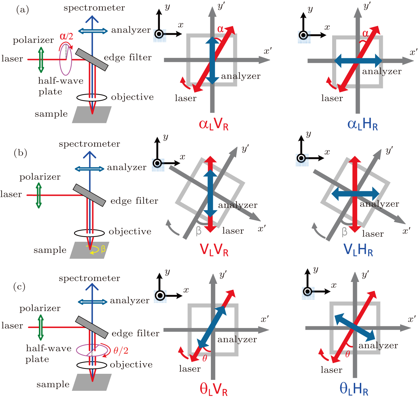
Fig. 1. (color online) Schematic diagrams of three typical polarization configurations for angle-resolved polarized Raman spectroscopy: (a) and , (b) and , and (c) and , in which the polarizer is set in the beam path to make the incident laser to be vertically polarized. The analyzer before the spectrometer entrance selects vertically or horizontally polarized Raman signal to be detected. The half-wave plate is used to change the polarization direction of laser or signal. Laboratory coordinate(xyz) is represented by black arrows while crystal coordinate ( ) is represented by gray arrows. Red two-way arrows stand for the incident laser polarization reaching at sample. The blue two-way arrows represent the original polarization of Raman signal corresponding to vertically or horizontally polarized signal selected by the analyzer before spectrometer entrance.
3. General analysis for three typical angle-resolved polarization configurations

The intensity of a Raman active mode with Raman tensor can be calculated by:

where is a Raman tensor[25] and are the unit polarization vectors of the incident laser and scattered Raman signal, respectively. A Raman mode may have multiple Raman tensors. The total Raman intensity I is obtained by the summation of Raman intensity from each Raman tensor .

Now we start to analyze the angle-resolved Raman intensity of the Raman active mode under the three typical polarization configurations. In the calculation, we consider an arbitrary Raman tensor for given in the corresponding crystal coordinates:

i) and

The incident laser propagates along axis with polarization vector . The Raman signal is backscattered along z axis with polarization vector fixed by the analyzer as for and for , respectively. Based on Eq. (1), Raman intensity of the arbitrary Raman tensor in the configurations and is

and

When rotating the sample in the xy plane, there is an angle between laboratory coordinates(xyz) and crystal coordinates ( ). Because the Raman tensors ( ) of a crystal are defined according to its crystal coordinates, it must be converted into laboratory coordinates ( ) by , where M is defined as a transform matrix linking the two coordinates:

Thus, Raman intensity is evolved into . The incident laser propagates along axis with polarization vector along y axis: . The Raman signal is backscattered along with polarization vector fixed by the analyzer as for and for , respectively. Based on Eq. (1), Raman intensity of the arbitrary Raman tensor in the configurations of and are

and

The half-wave plate inserted in the common optical path of incident laser and scattered Raman signal will simultaneously change the polarization directions of both two beams. To facilitate calculations, we introduce the Jones matrix of the half-wave plate in xy plane:[26]

where is twice of the angle ( /2) between its axis of the half-wave plate and y axis. The polarization of the incident laser is changed by half-wave plate when it reaches to the sample at which the laser polarization . The analyzer is positioned before the spectrometer entrance with for and for . is changed from at sample by the half-wave plate via . The Raman intensity under this configuration is , and the final result is as follows:

As shown in the expressions for configurations ii) and iii), is equivalent to while is equivalent to because in configuration ii) is corresponding to in iii). This illustrates that the polarization configuration to insert a half-wave plate in the common optical path of the incident laser and scattered Raman signal can be a substitution of the one to rotate the sample, which is more technically difficult and time-consuming than the former.

4. ARPR spectroscopy on the basal and edge planes of HOPG

We then verify the above results of ARPR experiment on the basal and edge planes of HOPG. HOPG is characterized by an arrangement of parallel graphene layers which can be treated as a modelling system of two-dimensional materials. It is highly oriented with respect to its layer-stacking direction. HOPG belongs to , 12 vibration modes at point are expected and denoted as:[27] . For pristine graphite, two doubly degenerate modes are detected ( , usually referred as the C mode) and ( , usually called G mode).[7,28] However, the position and intensity of the G mode in graphene is very sensitive to its doping level, and its G mode position can be located up to in CVD-grown graphene.[29] Raman scattering measurements are performed at the basal and edge planes of HOPG at room temperature and excited by a 532-nm laser. It is measured under back scattering configuration using a micro-Raman system (HR Evolution, Horiba Jobin Yvon) equipped with a edge filter and a charge-coupled device (CCD) detector. The spectra resolution is estimated to be about 0.53 per CCD pixel with an 1800 lines/mm grating. A 100 microscope objective (NA = 0.9) is used to focus the incident light and collect the scattered Raman signal. Samples are positioned on an XY piezostage or a rotation stage according to specific demands of polarization configurations. Laser spot has a diameter of m at the sample surface. The laser power kept below 1 mW to avoid sample heating.[30]

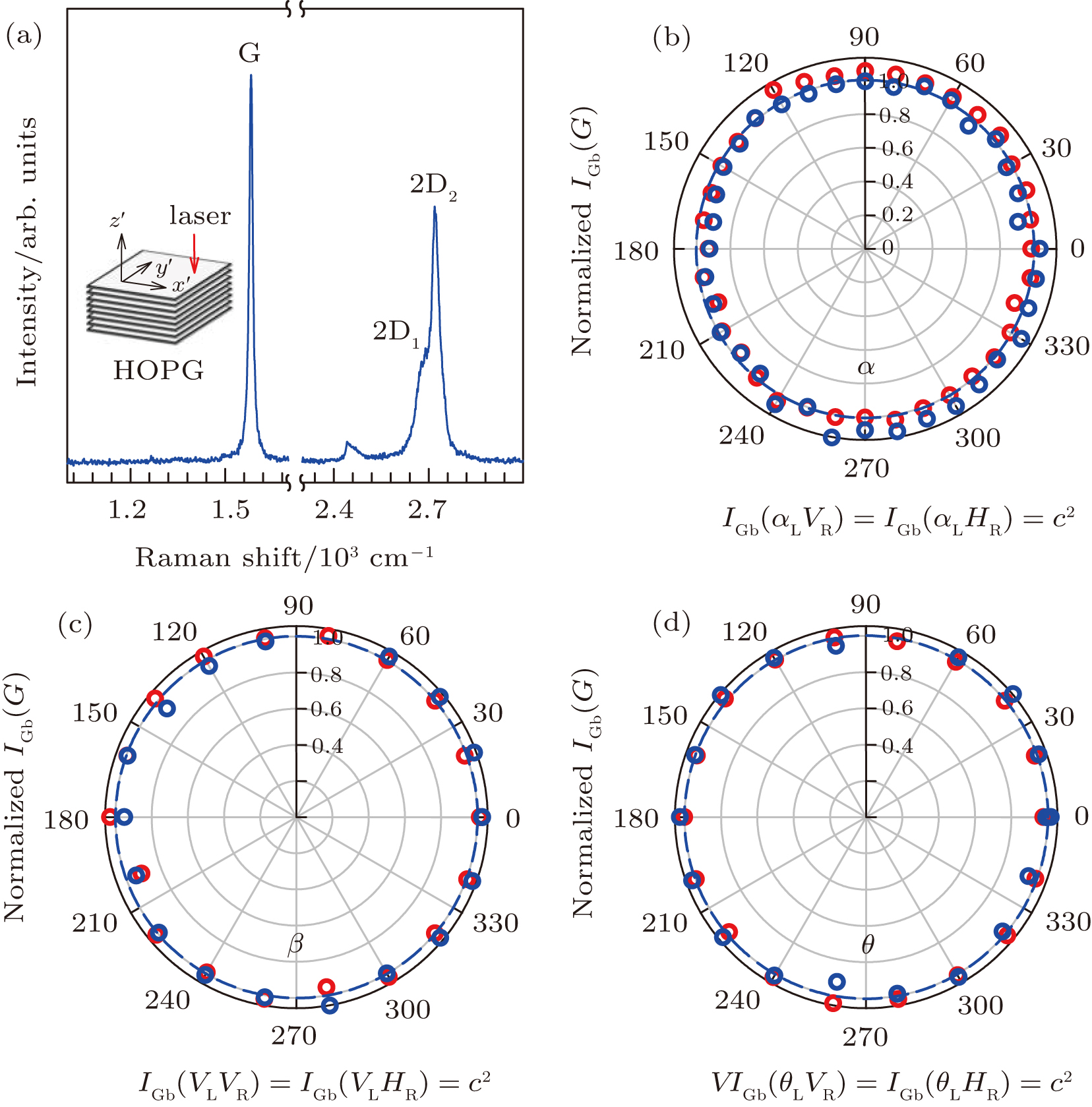
4.1. Angle-resolved polarized Raman measurement at the basal plane

Figure 2(a) presents the Raman spectrum measured on the basal plane of HOPG. The G, 2 , and 2 modes are observed.[31] The absence of D mode indicates that the sample is with high crystal quality.[31] We measured the G mode intensity at the basal plane ( (G)) of HOPG under the three polarization configurations as addressed above. The G mode has two Raman tensors ( , ):[25]

where c is a constant. Accordingly, the calculated in the three polarization configurations are listed in Table 1, and shown in Figs. 2(b)2(d) by dashed lines. All the remain a constant of , independent of laser polarizations and sample azimuth, manifesting itself as an isotropic material on its basal plane. We also plot the experimental results under the three polarization configurations as shown in Figs. 2(b)2(d) by red circles ( , , ) and blue circles ( , , ), respectively. When , , and increase from to , all the experimental in the three polarization configurations keep constants, in agreement with the theoretical results.

Fig. 2. (color online) (a) Raman spectra at the basal plane of HOPG. Inset shows schematic image of the basal plane for Raman measurement. (b) Polar plot of the G mode intensity at the basal plane as a function of for configurations of and . (c) Polar plot of as a function of the sample rotation angle for configurations of and . (d) Polar plot of as a function of laser polarization angle for configurations of and . The dash curves are the fitted results.
Table 1.

Calculated results of and under the three polarization configurations. Incident laser polarizations are shown in row while analyzer directions in column.

.
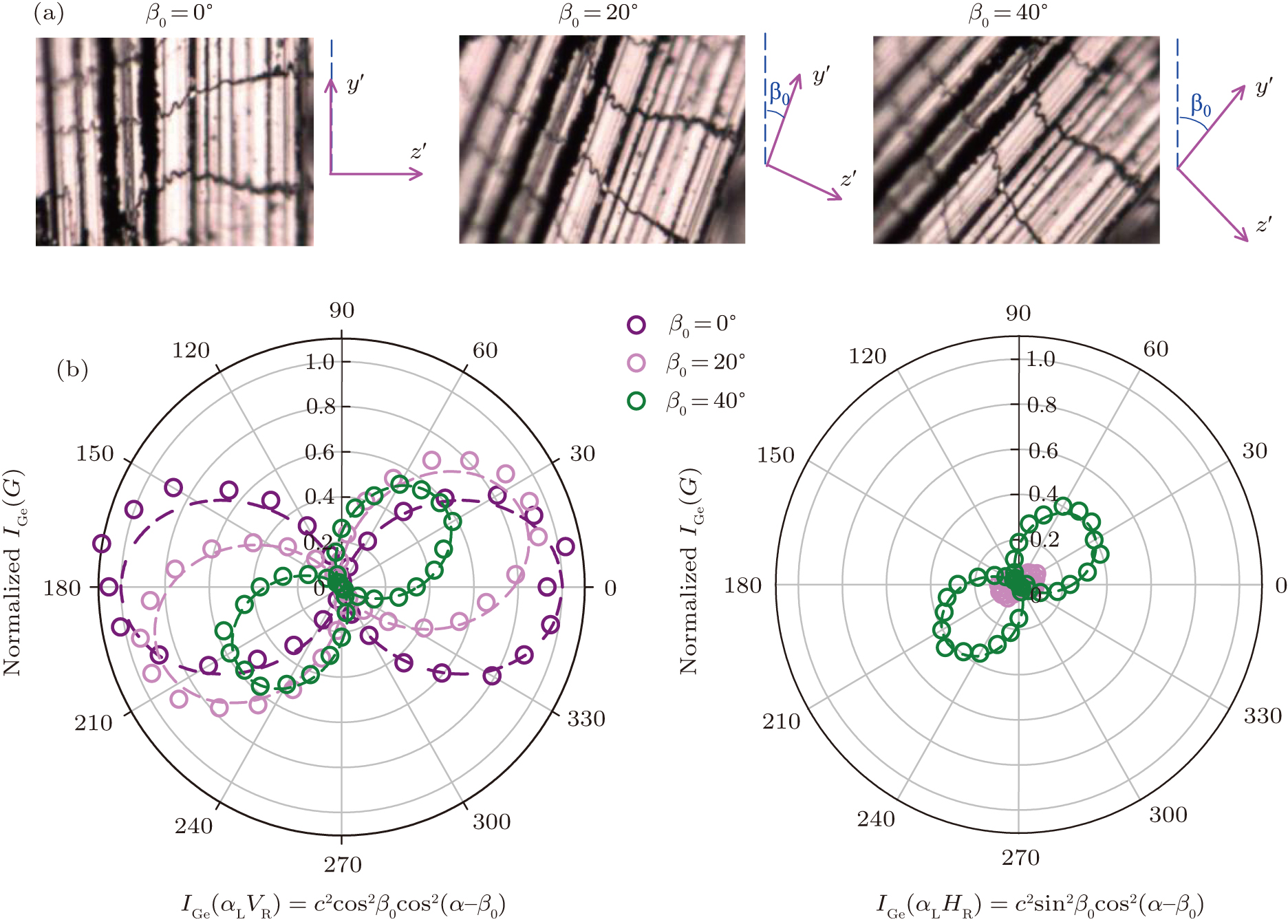
4.2. Angle-resolved polarized Raman measurement at the edge plane

Figure 3(a) presents the Raman spectrum measured at the edge plane of HOPG. Compared with the Raman spectrum at the basal plane, there are three extra first-order modes on the edge plane of HOPG at (1347.7 ), (1366.8 ), and (1627.4 ),[32] which are activated by intervalley and intravalley double resonant Raman scattering, respectively.[33] The Raman spectra of HOPG at the basal plane is in the absence of the D mode because of its high crystal quality, but the emergence of the D mode at the edge plane results from the presence of the edge. The edge-induced D mode at the basal plane is due to the in-plane breathing vibration of six-atom rings and comes from the TO phonons around the Brillouin zone corner K.[34]

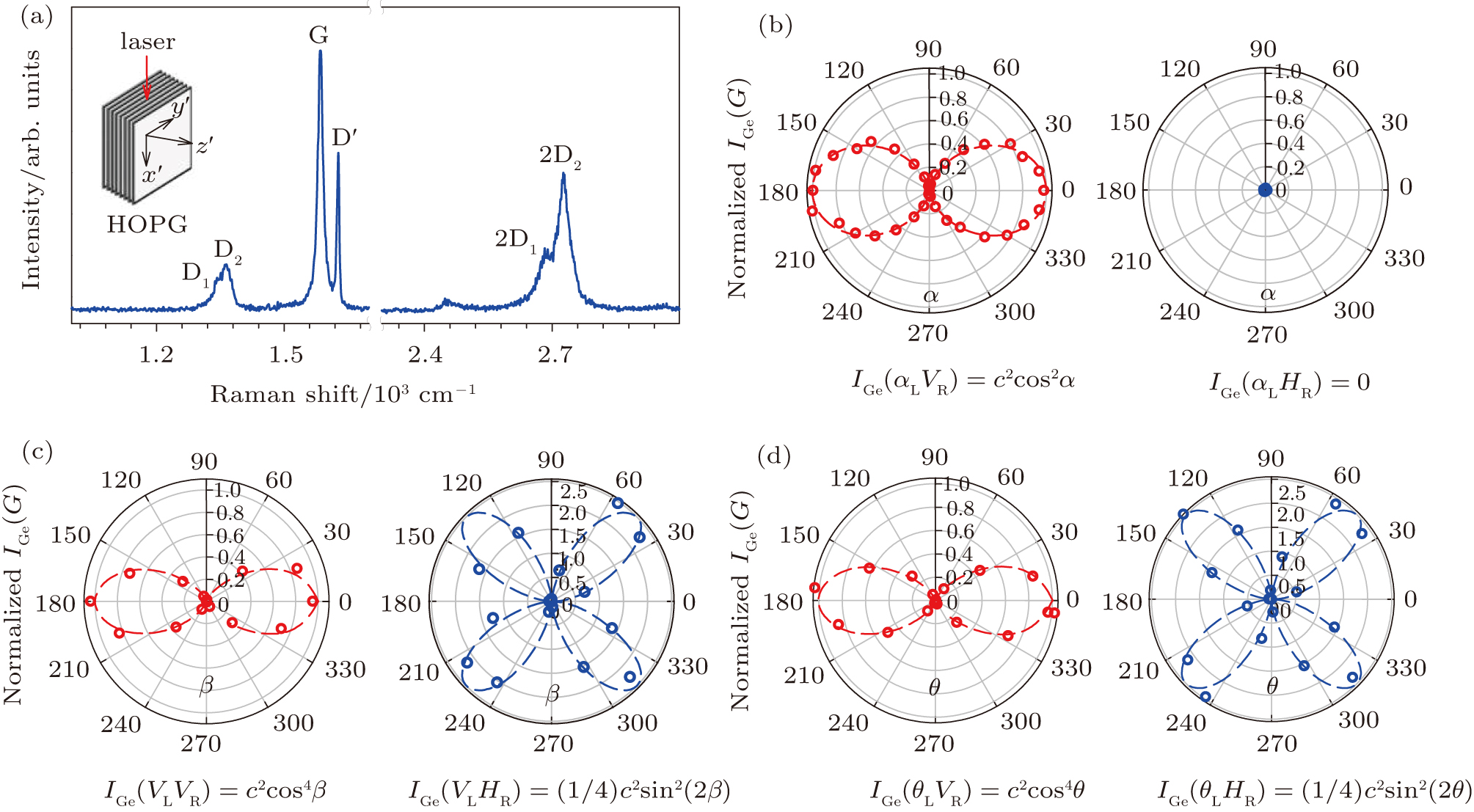
Fig. 3. (color online) (a) Raman spectrum of HOPG at the edge plane with incident laser and analyzer polarization along the axis. Inset shows schematic image of the edge plane for Raman measurement. (b) Polar plot of the G mode intensity at the edge plane ( ) as a function of laser polarization angle for configurations of and . (c) Polar plot of as a function of sample rotation angle for configurations of and . (d) Polar plot of as a function of laser polarization angle for configurations of and . The dash curves are the fitted results.

Since the above Raman tensor and are based on the basal plane, we must first obtain the Raman tensor on the edge plane. By rotating the sample along crystal coordinate axis by , Raman tensors ( and ) on the edge plane can be obtained as ( )

Based on and , we calculate the G mode intensity at the edge plane ( ) under the above three polarization configurations and summarize the results in Table 1. The corresponding angle-resolved are depicted in Figs. 3(b)3(c) by dashed lines. Except the zero of , all the measured are highly anisotropic. shows a maximum when the laser polarization is along graphite planes ( ). depends on and reaches the strongest intensity at and , i.e., the edge plane orientation lying along the laser polarization direction. However, displays four maximum when varies from to . The maximum intensity of is found to be four times as much as that of . As expected, in and is identical to the case in and , respectively. The above results actually indicate that HOPG at the edge plane is significantly anisotropic.

We also plot the experimental results of at the edge plane under the three polarization configurations by circles as shown in Figs. 3(b)3(d), respectively. The experimental results agree well with the theoretical ones, as clearly illustrated in Figs. 3(b)3(d). We also measured the polarization behavior of other three first-order modes , , and Dʹ at the edge plane of HOPG. The Raman intensity of , , and Dʹ modes follows an identical polarization feature to the G mode. In principle, the crystal translational symmetry is absence at the edge of HOPG, so the routine polarization analysis is not appropriate for the edge-induced D mode at the edge plane. The observed polarization behavior of , , and Dʹ modes may be that they are in-plane vibrational modes similar to the G mode. Anyway, the polarization behavior of the G mode at the edge plane can be well understood and the G mode is the intrinsic mode with strong intensity in HOPG, however, the , , and Dʹ modes are related with the crystal quality, disorder types, or edge orientation.[34] Therefore, their polarization behaviors are not discussed here, which is beyond the scope of this work.

The above result shows that reaches maximum when the laser polarization is parallel to the edge plane orientation. This feature can be used to determine the azimuth angle of HOPG. Assuming a pre-existing azimuth angle , under and configurations are expressed by: and . and reach maximum when and , i.e., the laser polarization paralleling to the edge plane orientation. With increasing sample azimuth angle from to , the maximum of decreases while increases. Figure 4(a) shows the optical images of three HOPG at the edge plane with of 0°, 20°, and 40°. The experimental results of and are presented in Figs. 4(b) and 4(c), respectively. It is worth while mentioning that the ratio of is a monotonic decreasing function of from to and independent of . If the of HOPG at the edge plane is unknown, it can be unambiguously derived from the ratio obtained experimentally. This can be utilized to precisely determine the orientation of graphene layers at its edge plane of HOPG.

Fig. 4. (color online) (a) Optical image at edge planes of HOPG with the pre-existing azimuth angle fixed at , 20°, and 40°. Laboratory coordinate y axis is shown in blue dash line. (b) Polar plot of as a function of laser polarization angle for , 20°, and 40°. (c) Polar plot of as a function of laser polarization angle for , 20°, and 40°. The dash curves are the fitted results with and .

Similar orientation-dependent Raman spectra has been proven to be of great use for thin ropes of single-wall carbon nanotubes[11] and bundled multiwall nanotubes.[12] They are highly orientation-dependent and reach maximum intensity of all Raman modes when the incident and analyzed polarization are aligned parallel to the nanotube axis and strongly suppressed when perpendicular, which is described as antenna effect.[35] This orientation judgment is obviously essential because their optimized properties always arise in their crystallographic orientation direction. In principle, the detailed analysis in this work reveals its promising applications for other 2D layered materials with anisotropic structures, i.e., vertically aligned multilayer graphene and Graphene-based films,[22,36] vertically standing transition metal dichalcogenides layered materials[18] and their heterostructures.[19] Indeed, polarized Raman spectroscopy had been applied to vertically standing two-dimensional flakes to determine whether the c axis of the vertically standing multilayer flakes are randomly distributed.[37] Angle-resolved polarized Raman spectroscopy can also determine the alignment angle of graphene and/or its chemical derivate graphene oxide in the free-standing films.[22] There is no requirement imposed on the thickness of each vertically standing flake of the samples.

5. Conclusions

In summary, we analyzed the ARPR intensity under three typical polarization configurations in detail for the Raman mode with a general Raman tensor. We demonstrated that the polarization configuration by rotating the sample orientation is equivalent to that by setting a half-wave plate in the common optical path of the incident laser and scattered Raman signal. The latter configuration can be preformed without rotating the sample, which makes the measurement more convincing, more technically easy to handle and time-saving than the former one. HOPG is used as a modelling system of two-dimensional materials for the analysis of ARPR intensity. The Raman intensity of the G mode at the edge plane exhibits an anisotropic behavior and reaches maximum when the polarization directions of both the incident laser and scattered Raman signal paralleling to its basal plane, which shows the potential application of ARPR spectroscopy for orientation determination of anisotropic and vertically standing 2DMs and other materials.[1317,38]

Reference
[1] Zhang X Tan Q H Wu J B Shi W Tan P H 2016 Nanoscale 8 6435
[2] Li X L Han W P Wu J B Qiao X F Zhang J Tan P H 2017 Adv. Funct. Mater. 1604468 http://dx.doi.org/10.1002/adfm.201604468
[3] Wu J B Zhang X Ijäs M Han W P Qiao X F Li X L Jiang D S Ferrari A C Tan P H 2014 Nat. Commun. 5 5309
[4] Lui C H Ye Z Keiser C Barros E B He R 2015 Appl. Phys. Lett. 106 041904
[5] Zhang X Han W P Qiao X F Tan Q H Wang Y F Zhang J Tan P H 2016 Carbon 99 118
[6] Zhao W J Tan P H Zhang J Liu J 2010 Phys. Rev. 23 245423
[7] Tan P H Han W P Zhao W J Wu Z H Chang K Wang H Wang Y F Bonini N Marzari N Pugno N Savini G 2012 Nat. Mater. 11 294
[8] Zhang X Han W P Wu J B Milana S Lu Y Li Q Q Ferrari A C Tan P H 2013 Phys. Rev. 87 115413
[9] Ji J T Zhang A M Yang R Tian Y Jin F Qiu X G Zhang Q M 2016 Chin. Phys. 25 067803
[10] Wei G N Tan Q H Dai X Feng Q Luo W G Sheng Y Wang K Pan W W Zhang L Y Wang S M Wang K Y 2016 Chin. Phys. 25 066301
[11] Duesberg G S Loa I Burghard M Syassen K Roth S 2000 Phys. Rev. Lett. 85 5436
[12] Rao A M Jorio A Pimenta M A Dantas M S Saito R Dresselhaus G Dresselhaus M S 2000 Phys. Rev. Lett. 84 1820
[13] Zhao H Wu J B Zhong H X Guo Q S Wang X M Xia F N Yang L Tan P H Wang H 2015 Nano Res. 8 3651
[14] Qiao X F Wu J B Zhou L Qiao J Shi W Chen T Zhang X Zhang J Ji W Tan P H 2016 Nanoscale 8
[15] Kim J Lee J U Lee J Park H J Lee Z Lee C Cheong H 2015 Nanoscale 7 18708
[16] Huang M Yan H Chen C Song D Heinz T F Hone J 2009 Proc. Natl. Acad. Sci. 106 7304
[17] Wang Y L Cong C X Qiu C Y Yu T 2013 Small 9 2857
[18] Kong D S Wang H T Cha J J Pasta M Koski K J Yao J Cui Y 2013 Nano Lett. 13 1341
[19] Yu J H Lee H R Hong S S Kong D Lee H W Wang H Xiong F Wang S Cui Y 2015 Nano Lett. 15 1031
[20] Cho S Y Kim S J Lee Y Kim J S Jung W B Yoo H W Kim J Jung H T 2015 ACS Nano 9 9314
[21] Zhai P F Liu J Zeng J Duan J L Xu L J Yao H J Guo H Zhang S X Hou M D Sun Y M 2016 Carbon 101 22
[22] Dai Z H Wang Y L Liu L Q Liu X L Tan P H Xu Z P Kuang J Liu Q Lou J Zhang Z 2016 Adv. Funct. Mater. 26 7003
[23] Ribeiro H B Pimenta M A de Matos C J Moreira R L Rodin A S Zapata J D de Souza E A Castro Neto A H 2015 ACS Nano 9 4270
[24] Yoon D Moon H Son Y W Samsonidze G Park B H Kim J B Lee Y Cheong H 2008 Nano Lett. 8 4270
[25] Loudon R 2001 Adv. Phys. 50 813
[26] Jones R C 1941 J. Opt. Soc. Am. 31 488
[27] Mani K K Ramani R 1974 Phys. Status Solidi 61 659
[28] Tan P H Wu J B Han W P Zhao W J Zhang X Wang H Wang Y F 2014 Phys. Rev. 89 235404
[29] Ping J L Fuhrer M S 2014 J. Appl. Phys. 116 044303
[30] Tan P H Deng Y M Zhao Q Cheng W C 1999 Appl. Phys. Lett. 74 1818
[31] Tan P H Deng Y M Zhao Q 1998 Phys. Rev. 58 5435
[32] Kawashima Y Katagiri G 1995 Phys. Rev. 52 10053
[33] Tan P H An L Liu L Q Guo Z X Czerw R Carroll D L Ajayan P M Zhang N Guo H L 2002 Phys. Rev. 66 245410
[34] Ferrari A C Basko D M 2013 Nat. Nanotech. 8 235
[35] Jorio A Souza Filho A G Brar V W Swan A K Unlu M S Goldberg B B Righi A Hafner J H Lieber C M Saito R Dresselhaus G 2002 Phys. Rev. 65 121402
[36] Liang Q Z Yao X X Wang W Liu Y Wong C P 2011 ACS Nano 5 2392
[37] Fu X L Qian J W Qiao X F Tan P H Peng Z J 2014 Opt. Lett. 39 6450
[38] Wu J X Mao N N Xie L M Xu H Zhang J 2015 Angew. Chem. Int. Ed. 54 2366