1. IntroductionThe birth of quantum mechanics is commonly attributed to the discovery of the Planck relation. In order to explain black-body radiation, Planck postulated that the radiation energy is transmitted in packages (“energy quanta”). Einstein later studied the photoelectric effect and found that the energy of light absorbed by an electron is also in small “packets”, which, like Planck’s “energy quanta”, is proportional to the light frequency ν.[1] This relation is now called the Planck relation or Planck–Einstein relation:
 |
The constant “h” here is called “Planck’s constant”. Subsequently, Planck’s constant was found to play a major role in many aspects of quantum physics, including the de Broglie relation p = hk; Dirac’s fundamental quantum condition:
 , and Heisenberg’s Uncertainty Principle
 .[2–4] It has become one of the most important universal constants in physics. But up to now, people still do not know the exact physical meaning of h. Planck’s constant is more like a fitting parameter; it is not derived based on first principles. In order to get a better understanding of the physical basis of Planck’s constant, in this work we suggest a useful approach to deriving h by using the Maxwell theory.
Investigating the physical origin of Planck’s constant is not only important for advancing our understanding of the foundation of quantum physics, but also relevant to the current study of cosmology. According to the Big Bang theory,[5] in the early day of the universe, it was filled with energetic photons. After the universe cooled down, these primordial photons became the cosmic microwave background (CMB) that we can detect today.[6] From the recent satellite measurements, the microwave detected in the CMB follows perfectly Planck’s law of black-body radiation.[7] Thus, the microwave radiation must obey
 . Does this imply that the microwave radiation is transmitted in the form of discrete particle?
It is obvious that the microwave is a wave packet of electromagnetic radiation. It cannot be regarded as a pointed object, since its wave length is quite long. Then, how is it explained that CMB satisfies Planck’s relation? We think the answer is that a particle does not need to be a pointed object; a wave packet can behave like a particle. This work is to show that this can be the case.
2. Original concept of
 according to Planck
When the concept of h was first proposed in 1900, Planck thought that the idea of energy quantization was “a purely formal assumption ⋯ actually I did not think much about it ⋯”.[8] Later, he tried to justify Planck’s relation by using a very complicated theoretical argument, which was hidden in cumbersome formulism of thermodynamics and statistical mechanics.[9] A more comprehensible treatment of Planck’s argument was put forward by Debye in 1910.[9,10] In the following, we will briefly review Planck’s derivation of h by using Debye’s cleaned-up version as outlined by John Slater.[9]
Planck’s theory was basically to treat the emitter in the black-body radiation as a linear oscillator,
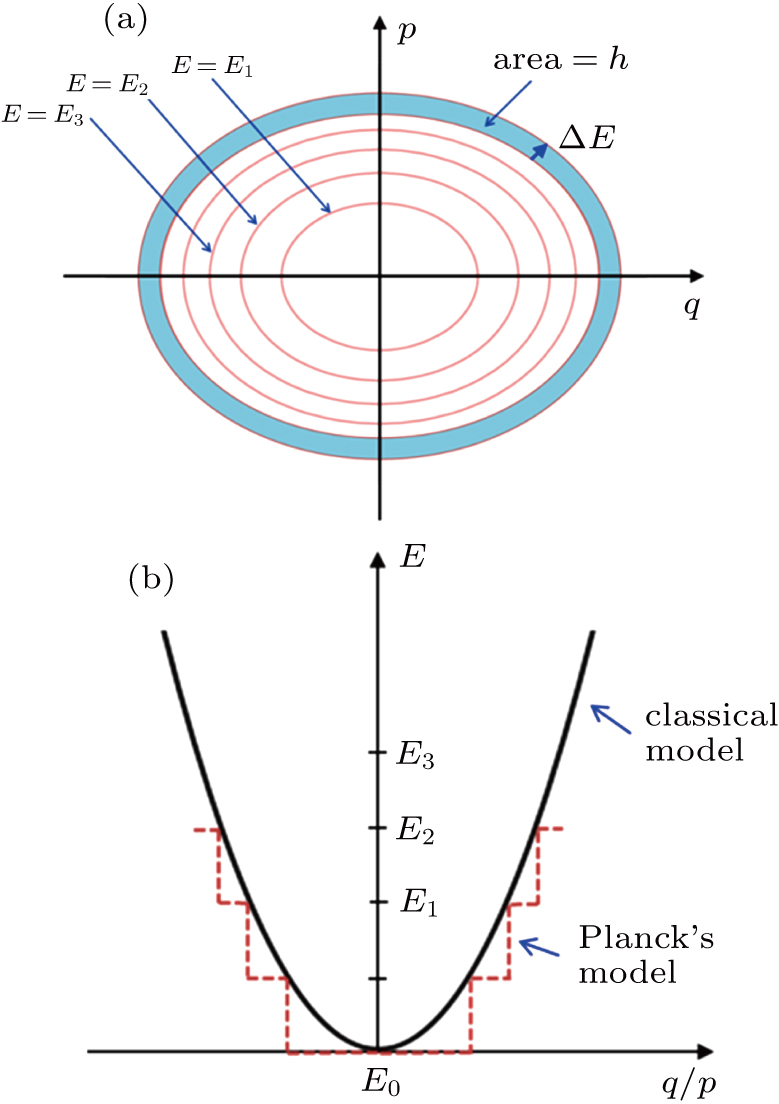
Here, E, T, and V represent the total energy, kinetic energy, and potential energy, respectively; q is the generalized coordinate and p is the generalized momentum; m and ω are the mass and frequency of the oscillator. If one maps the energy distribution in the phase space, one will find that the contour of a constant energy is an ellipse (Fig. 1(a)), since equation (2) can be reduced into
where

and
. The area enclosed by this ellipse is known to be
Then, when the energy is increased from E to
 , the corresponding incremental area in the phase space is (see Fig. 1(a))
Planck then made two formal assumptions:
With the above assumption, one can calculate the average energy of a black-body radiation emitter oscillating at frequency v by using the Boltzmann distribution, that is,
For simplicity, we denote
 ,
,
We know
and
Therefore,
Since we know that the number of energy states per unit volume and per unit frequency range in the radiation field is
 , the energy distribution in the radiator then is[9]
This equation is now known as “Planck’s law”. It fitted the experimental data of black-body radiation very well.[11]
Although the Planck law was a great success, Planck was not satisfied with the physical meaning of h as he derived it. Particularly, he knew that the assumption of partitioning the phase space (of the oscillator) into equal incremental areas is somewhat arbitrary. Planck spent subsequent years trying to justify his theory on better physical grounds but was not successful.[9]
3. Determination of energy and momentum carried by a photonIn this paper, we try to uncover the physical meaning of h by treating the photon as a wave packet of electro–magnetic radiation and directly calculating the total energy and momentum contained within the wave packet. More explicitly, the approach of this study is based on the following steps:
3.1. Energy density of an electro–magnetic fieldThe energy density of an electro–magnetic field is known to be[12]
where
ε and
μ are the dielectric permittivity and magnetic permeability of the vacuum,

and

are electric field and magnetic induction, respectively. According to Maxwell’s theory,

and

can be derived from the scalar potential

and the vector potential

:
 | (10a) |
 | (10b) |
In electro–magnetic radiation, the vector potential
 obeys the wave equation
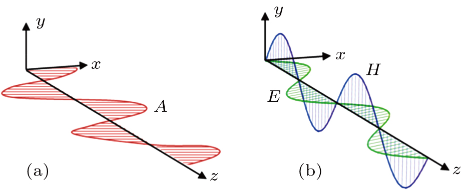
In order to calculate the energy density of an electro–magnetic wave, we choose a simple system in which the wave travels along the z axis and the vector potential is along the x axis (see Fig. 2), i.e.,
 , and
, and
Since there is no embedded charge within the vacuum,
 . Thus, equations (10a) and (10b) become
 | (13a) |
 | (13b) |
Substituting Eqs. (13a) and (13b) into Eq. (9), we have
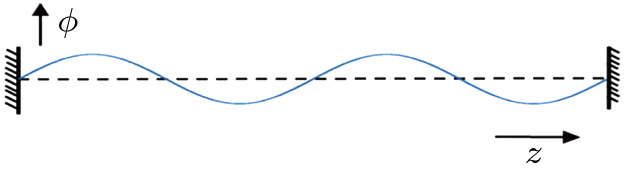
This relation suggests that Ax plays the role of the “field parameter” in wave propagation. This point can be easily seen by comparing Eq. (14) with the energy density equation in a one-dimensional (1D) stretched string (Fig. 3), which is
Here ρ is the mass density of the string, and F1 is the tension of the string.[13] One can immediately see that in the electro–magnetic system, Ax appears to play the role of a propagating field, just like the displacement ϕ in the stretched string.
Recall that the speed of light
 , one can directly calculate the energy density of the electro–magnetic system from Eqs. (12) and (14),
3.2. Total energy contained in a wave packet representing a photonTo find the physical meaning of Planck’s constant, we need to calculate the total energy
 contained within the wave packet representing one single photon. This energy can be obtained directly by integrating the energy density described in Eq. (16) over the entire volume of the wave packet:
 |
In order to carry out this integration, one must know the structure of a photon. In the literature, a photon is usually described by Eq. (12). This, however, is not strictly correct since it represents a continuous wave, which spreads over the entire space and time. The photon should have a limited size along its trajectory (z axis) and in the transverse plane (
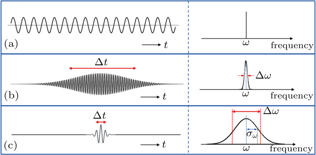
 plane). It should be a wave packet, which is constructed by the superposition of multiple wave components. Figure 4 shows three basic types of traveling waves: 1) a continuous wave, whose frequency is a fixed constant; 2) a wave packet with limited spread in the space and time dimensions (
 is very small); 3) a wave packet with a narrow spread over space and time (
 is very large). What does a photon look like? Since a coherent light (such as a laser) has a very narrow linewidth, the wave packet of a photon must be similar to that shown in Fig. 4(b). Such a wave function can be written as
where

describes the envelope of the wave packet. Since the photon travels in a straight line along the
z axis, we can assume that it has axial symmetry, i.e.,
where

and

are the transverse and longitudinal component, respectively. Equation (
18) then becomes
 can be constructed by superposition of plane waves with frequency slightly different from the central frequency (
 , i.e.,
where

is the frequency distribution function, which can be assumed to follow a Gaussian distribution with a standard deviation

, i.e.,
As is well known, the Fourier transform of Eq. (22) will also give a Gaussian distribution in the time domain. That is,
and
Once we know the envelope function in the time domain, we can easily obtain the envelope function in the spatial domain along the z axis,
where

. According to Eqs. (
16), (
17), and (
20), we can now calculate the total energy of the wave packet as follows:
Here
 and
and
 in Eq. (26) can be calculated separately as follows:
Recall that
 and
and
 ,
,

is known to be related to the linewidth (or half-width,

of the photon by
In most transmitting media, the linewidth of a wave is proportional to frequency ω. This ratio is defined as the “Q factor”,
The value of the Q factor is determined by the properties of the transmitting medium. Combining Eqs. (28), (29), and (30), we have
Substituting this into Eq. (27), and recalling
 , we have
Next, we need to calculate the value of
 . Its value can be easily determined if one knows the functional form of
 . As we have discussed earlier, the size of the wave packet in the transverse plane cannot be infinite. The simplest way to model
 is to assume that it has a constant value up to a cut-off radius (r0).
 then vanishes when
 . A more reasonable model, however, is to assume that
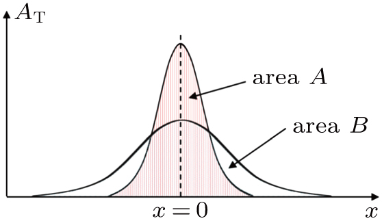
 follows a bell-shape Gaussian distribution (Fig. 5), i.e.,
where
a is the amplitude of the envelope function. From Eqs. (
26) and (
32), we have
This is closely related to the area of integrating the transverse component
 along the x axis, which can be called “ζ” (see Fig. 5(b)):
Combining Eqs. (33) and (34), we have
Substituting Eq. (35) into Eq. (31) and recalling
 , we obtain
Since
 represents the total electro–magnetic energy of a single photon, equation (36) is identical to Planck’s relation
 , and Planck’s constant h can be identified as
We will show later that
 has a clear meaning in quantum physics and should have a fixed cut-off value for a photon (see Section 4).
3.3. Total momentum contained in a wave packet: Justification of the de Broglie relationBy treating the photon as a wave packet of electro–magnetic radiation, we can also calculate the total momentum contained within the wave packet. As is well known, the energy flow of the electro–magnetic field can be described by the Poynting vector
 :[12]
:[12]
Since it can be shown that in a radiation system,
 , then,
From Eq. (16), we know
 , thus equation (39) becomes
 | (39a) |
The total energy flux of a wave packet of electro–magnetic radiation then is
For an electro–magnetic wave, the momentum density (
 is known to be related to the Poynting vector
 by[12]
Thus, the total momentum of a wave packet is
Substituting Eq. (40) into Eq. (42), and using Eq. (36), we have
Previously, we have already identified the value of h from Eq. (37). Recall that the wave vector
 , then equation (43) will become
Equation (44) shows that the total momentum of a photon is proportional to its wave vector
 . Equation (44) is identical to the de Broglie relation,[2]
Therefore, the Planck’s constant derived by us satisfies not only the Planck relation, but also the de Broglie relation.
4. Discussion4.1. Physical meaning of
 being a constant: The all-or-none principle
In the foregoing sections, we demonstrate that one can directly calculate the energy of a photon based on Maxwell’s theory. Based on this result, the Planck constant is given by Eq. (37).
Apparently, the Planck constant is dependent on the physical properties of the vacuum, e.g., the dielectric permittivity ε and magnetic permeability μ. The quality factor Q is also a property of the vacuum, since it is dependent on the transmitting medium. At this point, we do not know enough about the detailed properties of the vacuum to directly calculate Q. But the value of Q can be determined experimentally. One can use an optical device to directly measure the linewidth of a photon with known frequency. In the literature, there were already some hints about the value of Q. For example, it was reported that a solid-state dye laser (at 590 nm) could have a linewidth around 350 MHz.[14] This suggests that the Q factor is about 1.45
 106. Our work may motivate more accurate measurement of Q in the future.
The remaining problem is to consider whether ζ2 can be regarded as a constant and what that means. From Eq. (34), ζ is defined as the integrated area of the vector potential at the center of the wave packet. The requirement for ζ being a constant means that: Regardless of the oscillating frequency, in order to generate a sustainable oscillating wave, nature requires a critical amount of disturbance in the electro–magnetic field.
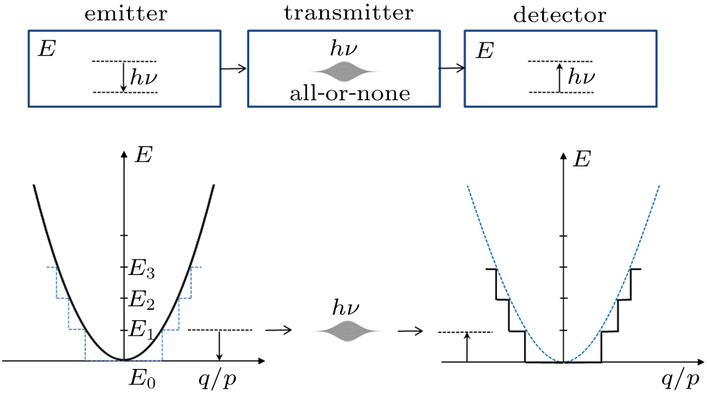
This situation is very similar to the generation of a nerve impulse. We know that a neuron can transmit a signal to its downstream target along its nerve fiber (called “axon”). This signal is called an “action potential”.[15] It is well known that the generation of action potential has the “all-or-none” property. That means that when the stimulus to the axon is below a threshold, no action potential can be generated. But when the stimulus is higher than the threshold, a full size action potential will be generated. This action potential will propagate along the axon with constant amplitude (about 100 mV).[16] In other words, one cannot generate an action potential with an arbitrarily small amplitude. And, no matter how large the stimulus is, one cannot generate an action potential which is much larger than 100 mV. That is why it is called “all-or-none”.
As it turns out, this all-or-none principle is applied in multiple aspects of nature. Not only the transmission of a nerve impulse is all-or-none, the transmission of the electro–magnetic radiation is also all-or-none. The radiation energy is apparently transmitted in small packets (photon), each of which has a limited size and is not sub-dividable. One can generate either a full size photon, or no photon at all. In other words, if the energy of the electro–magnetic field is smaller than a critical value, it will not be able to trigger a transmissible excitation wave traveling as a wave packet. Instead, the energy will just dissipate in the surrounding.
This requirement of “all-or-none” means that ζ should have a fixed cut-off value; it cannot be arbitrarily small. Thus, although the size of the wave packet is not fixed, the total amount of disturbance in the electromagnetic field (as measured by
 ) is fixed (see Fig. 6). If the diameter of the wave packet is very small, the oscillation amplitude of the electro–magnetic field within the wave packet must be large enough to make ζ reach the threshold value. Alternatively, if the oscillation amplitude of the wave packet is small, the size of the wave packet must be large enough to compensate it so that the integrated area reaches the threshold value.
Besides the above considerations, there is another reason for suggesting that ζ2 should be a constant. Recall that ζ2 was defined by Eq. (35). As we pointed out earlier in subSection 3.1, the vector potential (
 ) in an electro–magnetic radiation system is equivalent to the amplitude of an oscillation wave in a 1D vibrating string. Thus, if one wants to write down the wave function of a photon (
 , one can guess that ϕ must be related to
 (with a normalizing factor). Since the absolute square of the wave function
 is usually interpreted as the probability of finding the particle, this suggests that the absolute square of the vector potential of the wave packet,
 , is proportional to the probability of finding the photon. Recall that
 at the center of the wave packet, where
 , then one will be able to interpret
 | |
as a measure of “the total probability of finding the photon at the center of the wave packet”. So long as the wave packet represents a single photon, this probability should remain constant as the wave packet travels along the trajectory of the photon. Thus, the requirement for

being a constant essentially means that in an optical measurement, the probabilities of finding the photon at the center of the wave packet are always the same.
4.2. Reconciliation with Planck’s original modelNext, we examine whether our wave packet model is compatible to Planck’s original thinking. In the original work of Planck, his proposal of
 in black-body radiation was based on two assumptions: (i) the emitter can be modeled as a linear oscillator; (ii) the energy distribution of this oscillator somehow exhibits a step-wise pattern (blue dash lines on the left panel in Fig. 7). There were the following two problems in this model:
Now, with the findings of this paper, we can explain why Planck’s model could give the correct result. In the black-body radiation, the emitter gives out radiation waves which will be absorbed by the detector. If one accepts that the radiation wave is transmitted in wave packets, our calculation shows that the group energy of each wave packet is proportional to its oscillation frequency, i.e.,
 | (36a) |
In Planck’s model, the energy distribution of an emitter is modeled as a linear oscillator. It has a parabolic shape (see Fig. 7). The emission of a wave packet depends on the energy transition from a higher energy state to a lower energy state of the emitter. When the energy state of the emitter is less than
 above the ground state, it is incapable of giving off a photon at frequency v. That means that if one tries to detect the radiation signal from the emitter, one will fail to detect any photon emission (at frequency
 . This situation changes only when the energy level of the emitter reaches
 or above. Thus, if one studies the black-body radiation at a single frequency ν, there is no transmission of radiation energy from the emitter to the detector until the emitter reaches E1, where
 . Similarly, the emitter can be detected to emit two photons when the emitter reaches E2, where
 . This explains why the emission of a photon is a step-wise process when the energy of the emitter increases. (For more details, see Fig. 7.)
Thus, even though Planck did not calculate the energy content of a radiation wave packet, he could still correctly explain the black-body radiation by using a step-wise energy distribution model. All that he needed to do was to assume that the energy released from the emitters is in packets, which he called “energy quanta”.
4.3. Implications on the physical meaning of Heisenberg’s uncertainty principleOnce we can derive Planck’s relation and de Broglie’s relation based on the wave packet model, Heisenberg’s uncertainty principle can be easily explained. If one accepts that a photon is a wave packet of oscillating electro–magnetic field, which follows a Gaussian distribution along the particle trajectory, the half-width of the wave packet in the time domain can be directly determined from the linewidth of the radiation wave. From the condition of Fourier transform, we know
 , i.e., Eq. (24), where
 and σt are the standard deviations in the frequency domain and the time domain, respectively. Since we know that the half-width of the wave packet is
 and the linewidth of the oscillation frequency is
 , equation (24) implies
 . From Planck’s relation,
 , we have
This suggests that the product of linewidths in the energy and time domains for a single photon is very close to h. Such a result is consistent with Heisenberg’s conjecture that
Thus, Heisenberg’s uncertainty principle can be interpreted as a direct result of the fact that a photon is a wave packet which follows a Gaussian distribution.
Using this wave packet model, we can also easily obtain the uncertainty principle between
 and
and
 . Recall from the de Broglie relation,
 , then the half-width of the wave packet will be
 . From the conditions of the Fourier transform,
Then, the above relations give
This is consistent with the conjecture of Heisenberg that
 .
.
4.4. Other discussionThis work represents an approach of using a classical theory to explain the physical basis of h. What we have done so far is to derive Planck’s relation by calculating directly the energy contained within a wave packet based on Maxwell’s theory. Using such an approach, we can also derive the de Broglie relation and Heisenberg’s uncertainty principle. These derivations are straight forward and only based on a simple assumption that the photon is a wave packet of electro–magnetic radiation.
Since Planck’s constant is a fundamental physical constant, it is involved in many areas of study, including the foundation of quantum mechanics,[3,17] quantum field theory,[18,19] the study of chaos,[20] and tunneling,[21] etc. There have been many previous attempts to explain the physical basis of Planck’s constant.[22–26] For example, Galgani and Scott tried to use a classical mechanical model of a 1D particle chain to explain Planck’s relation.[22] They assumed a Lennard–Jones interaction existing between the nearest-neighboring particles and solved the classical equations of motion numerically. For a broad class of initial conditions, Planck-like distributions are obtained for the time averages of the energies of the normal modes. They reported that the action constant entering into such a distribution is of the same order of magnitude as Planck’s constant.[22]
In another study, Ross proposed a possible way of building Planck’s constant into the structure of space-time.[24] This was done by assuming that the torsional defect that intrinsic spin produces in the geometry is a multiple of the Planck length. He showed that by using a simple geometrical assumption, it could lead to the quantization of angular momentum. He thought that such an approach could be considered as a first step to derive the value of
 .
.
As an extension of Ross’s study, Duan et al.[26] proposed a new geometrization of Planck’s constant in terms of vierbein theory.[27] They thought that h is also connected with the defects of space-time. A set of invariances including the
 -like gauge transformations was used in this geometrization. Using the gauge-potential decompositions, the quantity introduced in this geometrization to describe the defects would be quantized. Such an approach would allow one to relate the Planck constant to the space-time defects.
All these previous attempts, however, involve very special assumptions which cannot be directly tested experimentally. Also, they cannot give the explicit value of Planck’s constant, as we did in Eq. (37). In our case, the derivation is based strictly on Maxwell’s theory, which is well established and already well supported experimentally.
Recently, quantum communication has become an important new field.[28,29] Obviously, the physical origin of the Planck constant has tremendous importance in this area of research. Since h essentially determines the size of a bit of information in quantum communication, it is very important to know the physical basis of the Planck constant. Thus, this work will be helpful to the further development of this field.


