Li Yang, Wang Sheng-Qian, Rao Chang-Hui. Error analysis of the piston estimation method in dispersed fringe sensor. Chinese Physics B, 2017, 26(3): 039501
Permissions
Error analysis of the piston estimation method in dispersed fringe sensor
Li Yang1, 2, 3, Wang Sheng-Qian1, 2, Rao Chang-Hui1, 2, †
Laboratory on Adaptive Optics, Institute of Optics and Electronics, Chinese Academy of Sciences, Chengdu 610209, China
Key Laboratory on Adaptive Optics, Chinese Academy of Sciences, Chengdu 610209, China
University of Chinese Academy of Sciences, Beijing 100049, China
† Corresponding author. E-mail: chrao@ioe.ac.cn
Abstract
Dispersed fringe sensor (DFS) is an important phasing sensor of next-generation optical astronomical telescopes. The measurement errors induced by the measurement noise of three piston estimation methods for the DFS including least-squared fitting (LSF) method, frequency peak location (FPL) method and main peak position (MPP) method, are analyzed theoretically and validated experimentally in this paper. The experimental results coincide well with the theoretical analyses. The MPP, FPL, LSF are used respectively when the DFS operates with broadband light (central wavelength: 706 nm, bandwidth: 23 nm). The corresponding root mean square (RMS) value of estimated piston error can be achieved to be 1 nm, 3 nm, 26 nm, respectively. Additionally, the range of DFS with the FPL can be more than 100 μm at the same time. The FPL method can work well both in coarse and fine phasing stages with acceptable accuracy, compared with LSF method and MPP method.
The next-generation optical astronomical telescopes mostly use segmented primary mirrors. Therefore, the piston errors (optical path difference) between different segmented mirrors will exist, and the assemble errors is usually larger than one wavelength; this will remarkably reduce image quality and should be less than 1/20λ.[1–4] In addition, the piston errors caused by the working environment must be measured online in real time. The dispersed fringe sensor (DFS) was proposed for these factors,[5] the experiments demonstrated that the DFS is an efficient and robust method for coarse phasing of segmented primary mirrors.[1] The NIRCam of James Webb Space Telescope (JWST) measured larger piston error by using the DFS, the range of detection is about ±300 μm. The piston errors of segmented mirrors can be reduced to less than about 300 nm for the JWST by the DFS.[6] The phasing camera of the Giant Magellan Telescope (GMT) also uses the DFS to measure the piston errors for coarse phasing, the phasing camera has a ±50 μm capture range and can reduce piston error to smaller than a root mean square (RMS) value of 120 nm.[7]
The accuracy of dispersed fringe sensor is determined by internal optical calibration error, wavefront error, and image quality of detector.[8] Spechle et al. presented an advanced DFS; an algorithm allows the overall method to be less sensitive to calibration errors.[8] Van et al. proposed an improved method to reduce the requirement for wavefront aberration, and simulation shows that this method can improve sky coverage.[9] There is no discussion about the image quality of the detector and estimation method is more applicable and practical, which are the focuses of this paper.
The DFS is a modified structure of Young’s Double-Slit Interference.[7] It uses dispersed element to modulate the interference light with piston error, and dispersed element spreads the light according to its wavelength, forming a spectrum on the camera. The piston errors of the segment mirrors will result in the intensity modulation in the dispersion direction.[5] The intensity is approximately described as a sine curve,[10] and the interference pattern along the interference direction is also affected by the piston error.[9,11,12] At present, several methods have been proposed to extract the piston error from a dispersed fringe image. According to the intensity in the dispersion direction, Shi et al. used least-squared fitting (LSF) to fit the frequency of the curve of the intensity versus frequency to determine the piston error (least-squared fitting method, LSF),[1] and the dispersed fringe sensor of the JWST used this method.[10] The dispersed fringe sensors in the phasing camera of the GMT obtains obtained estimation piston errors with frequency peak location method (FPL),[9] this method is also bases based on the frequency of the curve of the intensity versus frequency on in the dispersion direction, but it estimates the piston error form frequency information of the curve in the two-dimensional frequency domain of the dispersed fringe. Zhao and Cao,[11] and Zhang et al.[12] used the main peak position (MPP) method to estimate the piston error. Young’s double-slit interference is the foundation of this method, the main peak position in the interference direction has approximately linear relationship with the piston error.[9]
Therefore, different piston error estimation methods for dispersed fringe sensor have different error transfer processes of the noise in the dispersed fringe image. There are no analyses on the piston measurement error induced by the measurement noise. This paper concentrates on the estimation error caused by noise, when using different estimation methods to estimate piston error. The relation between the estimation error and noise is analyzed and experimental results accord well with the theoretical analyses. At the same time, the experiment shows that the first moment centroid calculation method can promise the accuracy of estimation result by using the FPL method, whether in coarse phasing or fine phasing. According to these results, the researchers or engineers can choose appropriate estimation method for the dispersed fringe sensor and optimize parameters of estimation method of dispersed fringe sensor.
This paper is divided into four parts. In Section 2, the relationship between the estimation errors of different methods to estimate piston error and the noise are analyzed. In Section 3, we describe the experimental system and procedure. In Sections 4 and 5 we describe our experimental results and present our conclusions, respectively.
2. Relation between the estimation error and noise
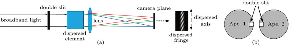
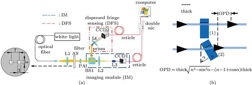
As shown in Fig. 1(a), a dispersed fringe with piston error is generated in camera plane, when the broadband light comes from two segmented mirrors with piston error. The double slit of the DFS superposed on the two segmented mirrors (Ape. 1 and Ape. 2) is shown in Fig. 1(b).
Fig. 1. (color online) (a) A representative structure of dispersed fringe sensor; (b) the double slit of the dispersed fringe sensor superposed on two segmented mirrors (Ape. 1, Ape. 2) of telescope.
As the general descriptions of the dispersed fringe by different phenomena, many methods can be used to calculate piston error,[5,9,11,12] which include the LSF, FPL, and MPP.
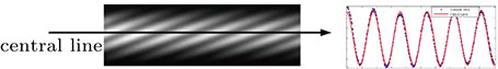
For the dispersed fringe image with piston error, the intensity along the dispersed axis is periodically changed, and the cycle has monotonic relationship with the piston error as illustrated in Fig. 2. The LSF and the FPL estimate the piston error based on this characteristic.
Fig. 2. (color online) The process of extracting piston error by using LSF method.
The intensity at the central line along the dispersion can be written as the following fundamental equation for convenience:[1]
(1)
where is the invariable amplitude, γ is the fringe visibility, δ is the piston error, and is the wavelength of the dispersed fringe along the dispersed direction. Equation (1) indicates that piston error modulates the period of intensity in dispersed axis. Therefore, the period of dispersed fringe can be obtained by fitting the curve of intensity versus frequency along the dispersion, and then the piston error can be estimated. This method is called LSF method, and it is indirect to calculate the piston error. In this method, least squares fitting algorithm is usually used to fit the period of dispersed fringe, and equation (1) approximates the sine function to fit the frequency of fringe.[5,10] Therefore, the piston error δ is calculated by the LSF method.
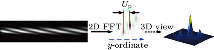
The change of intensity cycle at the dispersed axis also influences absolute value of the Fourier transform of the dispersed fringe,[9] another estimation method (FPL) is based on this point; the process of the FPL method for estimating the piston error is illustrated in Fig. 3.
Fig. 3. (color online) The FPL method estimated piston error form dispersed fringe.
As shown in Fig. 3, in the Fourier transform of dispersed fringe with piston error, the location () of the side lobe changes linearly with piston error in the y axis.[9] So, the piston error δ can be calculated by
(2)
where is the coherent length of the light.
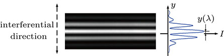
Along the interferential direction which is perpendicular to the dispersed axis, the change of the intensity accords with double-slit interference regulation as shown in Fig. 4. The MPP estimates the piston error by using this principle.
Fig. 4. (color online) The MPP method in which the position of the main peak is used to determine piston error.
As shown in Fig. 4, the main peak in the interferential direction deviates from the ideal peak location when two light beams of Young’s double-slit interference have piston error. The offset distance y(λ) and piston error (δ) are related by
(3)
where T(λ) is the spacial cycle of the interference pattern along the y axis in Fig. 4. Thus, the piston error can be calculated from Eq. (3), and it has a very good linear relationship with this kind of changing.[9]
2.1. Estimation error of the least-squared fit method
This method based on the intensity along the dispersion is approximately described as a sine curve, and the frequency of the curve has monotonic relationship with piston error. According to this phenomenon, the piston error can be estimated from the frequency of the curve which is fitted by the LSF algorithm. The photon noise is a Poisson distribution in the condition of small photon counts, while the DFS works in the environment with larger counts, the photon noise can be considered as Gaussian noise.[14] At the same time, this will make analysis easier. All of the following analysis is based on this prerequisite. There are two different least square methods to calculate the parameter of signal, one is the three-parameter sine-fitting algorithm, and the other is four-parameter sine-fitting algorithm.[15] When the sampling rate is high enough, the fitting errors of two different algorithms can be ignored.[16] When signal data is contaminated by Gaussian noise, the maximum and minimum values of fitting error have the relationship with noise[16]
(4)
where the variance of error of fitting frequency is , is the variance of the noise, A is the amplitude of light intensity, and M is the sampling rate.
For the dispersed fringe sensor, when the bandwidth is far less than the central wavelength, equation (1) can be rewritten as
(5)
where , with being the coherent length of the light.
Therefore, piston error can be calculated by
(6)
Then, the frequency f has the following relationship:[15]
(7)
where s, A, M, and φ are the estimated sine-wave parameters.
From Eqs. (6) and (7), the error () of fitting frequency and estimation error of the piston error are related together, the variance of the estimation error is
(8)
Therefore, the bounds of variance for estimation error are shown, respectively, as follows:
(9)
2.2. Estimation error of the frequency peak location method
In absolute value of the two-dimensional Fourier transform of the dispersed fringe, the location of the side lobe changes linearly with piston error in the y ordinate. Therefore, the error caused by noise would be introduced into the process of extracting the location or position of the side peak in the frequency domain.
When the centroid position () of side peak in the two-dimensional image is detected by using the first moment centroid calculation method[17]
(10)
where M and L are the numbers of pixels in the two-dimensional direction, respectively, is the intensity of pixel location at , and is the coordinate of the pixel. The variance of estimated location error () caused by the noise in the fringe image is[17]
(11)
where is the sum of the intensity of sub-window,, and is the variance of error sources of (i, j)th pixel. Since the Fourier transform of a Gaussian is also a Gaussian,[18] the noise in the frequency domain of an image with Gaussian noise is of Gaussian distribution. The variance () of Gaussian noise in the pixels of the Fourier transform is similar, , and we have[18]
(12)
where is the ideal position of image spot in the sub-window. When the ideal position of image spot is set to be a reference value, here ,
(13)
When extracting the centroid position of side peak in frequency domain, one-dimensional intensity along the locomotive direction is enough to estimate the location, because it contains all the information about the piston error. Hence, according to Eq. (13), the estimated location error can be obtained by
(14)
Substituting Eq. (2) into Eq. (14), the estimation error () of piston error affected by noise can be obtained as follows:
(15)
2.3. Estimation error of the main peak position method
When the piston error is calculated from Eq. (3), the location or position of main peak should be extracted first, and then the offset distance can be obtained. In this process, noise has an influence on extracting the position of main peak, and then it will affect the result for calculating the piston error.
The MPP method only uses intensity in the interferential direction, in which the process of extracting the centroid position is the same as that of the FPL, and we have centroid detection error, which can be expressed as
(16)
According to Eq. (3), the standard deviation of estimation error caused by noise is
(17)
3. Experiment
The experimental layout is shown in Fig. 5, in which the white light plane wave is formed by L1 (lens), aperture stop (AS) with double stilt transforms plane wave into dual-beam, and the dual-beam is adjusted by the phase adjuster (PA)[7] to generate relative optical path difference. The PA can easily generate controllable static piston error of segmented telescope and is used in prototype phasing camera for the GMT.[7] Therefore, there is no need to use segmented mirrors nor telescope to generate piston errors. Finally, the beam splitter prism (BS1) reflects the beams into the dispersed fringe sensor and dispersed fringe image is captured by the CCD2 camera (Baumer TXG12).
Fig. 5. (color online) Layout of the experiment. (a) The experimental setup, (b) the principle sketch of the phase adjuster.
The dispersed fringe image with a resolution of 500×40, the pixel size of the camera is 3.75 μm. The bandwidth of light is 23 nm with a central wavelength of 706 nm, and these can be changed by light source (NKT Superk). Residual surface error of plane wave is λ/10 peak value (PV), the dual-beam generated by the double stilt, therefore the wavefront distortion has a limited effect on dispersed fringe image. The angular calibration error between the camera and the dispersed element is less than ±5 (see Fig. 6). The equivalent piston error is also less than 3‘nm. Therefore, the optical calibration errors and wavefront errors are very small and the experimental setup can ensure the correctness of the experimental data.
Fig. 6. (color online) Calibration error of the dispersed fringe sensor detected with calibration software.
In the experiment, several groups of dispersed fringe images are generated by the DFS in different noise conditions by changing the mean ADU (the minimum unit of digital readout from A/D converter) and standard deviation of background noise. And then, for each group different estimation methods are used to calculate piston errors of the dispersed fringe images in the same noise condition. The noise effects on the accuracy of different estimation methods can be compared with the standard deviation of these piston errors. The result of the experimental error accords well with the theoretical calculation, and the correctness of the theoretical expressions are verified.
4. Results
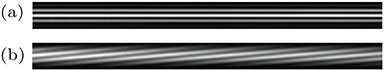
The LSF is suitable for calculating large piston error (larger than one wavelength), and the MPP can only estimate the fraction of piston error (less than one wavelength),[11,12] so two kinds dispersed fringe images with different piston errors are used to calculate the errors. As shown in Fig. 7, there are two sorts of dispersed fringes with small piston error (about 7 nm) and large piston error (about 123.3 μm), respectively.
Fig. 7. Reference dispersed fringe images. (a) The fringe with small piston error; (b) the fringe with large piston error.
There are 20 groups of dispersed fringe image set with the same light signal intensity, but their signal-to-noise ratios (SNRs) are different. In each group of dispersed fringe images, the standard deviation of the noise in the dispersed fringe imageis approximate. The standard deviation of noise increases with the serial number of image groups linearly. Consequently, the SNR is increased. The standard deviation of piston error is increased from 1 to 20 ADU, and the step size is 1 ADU.
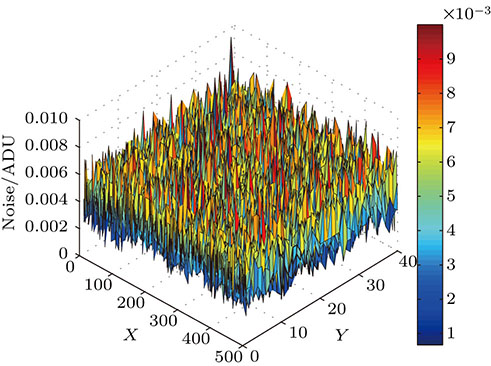
Figure 8 shows the noise amplitude of the reference fringe image. The noise amplitudes are all less than 0.01 ADU in each single pixel; this value is much less than the variance of noise in the noise-polluted images. Therefore, all the experimental results are given by using the peak-signal-to-noise-ratio (PSNR).[19]
(18)
where peakval is the maximum signal value that exists in a reference image (here ), and MSE is the mean square error between images with noise and reference image.
Fig. 8. (color online) Noise amplitude of reference fringe image, x and y are dispersed axis and interferential axis in the dispersed fringe image, respectively.
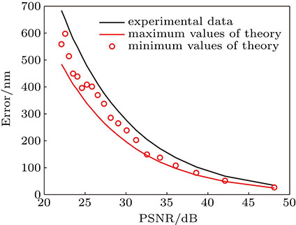
The characteristic curves of the error for the LSF in different noise conditions are shown in Fig. 9, when the LSF is used to estimate the piston error of dispersed fringe image with large piston error. The theoretical values are calculated by Eq. (9), where /ADU, M = 500, and .
Fig. 9. (color online) Experimental errors and theoretical errors obtained by using the LSF in different noise conditions of dispersed fringe images with large piston error.
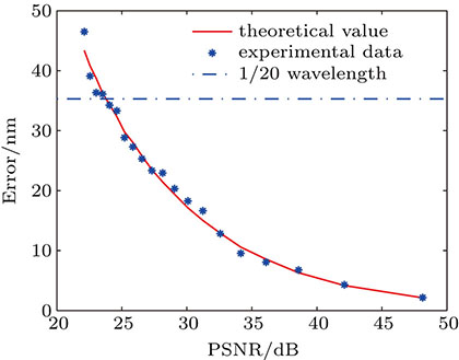
Figure 10 show the measured error of the FPL in the different noise conditions, when the FPL is used to estimate the piston error of dispersed fringe image with small piston error and a resolution of 500×40 pixel. The theoretical values are calculated by Eq. (15), where , , and L = 10 for the FPL.
Fig. 10. (color online) Experimental errors and theoretical errors obtained with the FPL, when dispersed fringe images with small piston error are used.
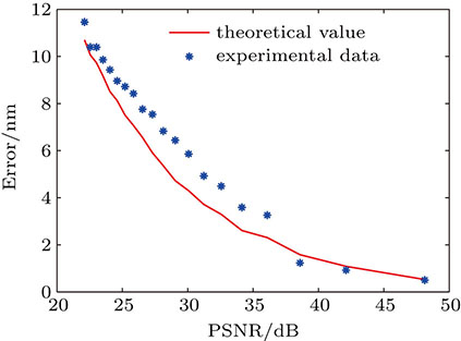
The result of the MPP method is illustrated in Fig. 11. The theoretical values are calculated by Eq. (17), where , , and L = 8 for the MPP.
Fig. 11. (color online) Experimental and theoretical errors obtained with the MPP, when dispersed fringe images with small piston error are used.
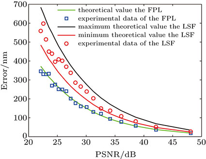
In the casewhere there are two kinds of dispersed fringe images with different piston errors, the FPL is compared with the LSF by using dispersed fringe image with large piston error and a resolution of 500 in dispersed direction. The theoretical values of the FPL are calculated from Eq. (15), where , , and L = 10 for the FPL.
As seen in Fig. 12, the measurement errors of the FPL and the LSF are approximate. The measured errors of two different methods have similar results in identical condition.
Fig. 12. (color online) Comparison of the FPL with the LSF by using dispersed fringe images with large piston error, the window width of FPL in frequency domain is 10 pixel.
5. Conclusions
In this paper, we analyze the accuracy provided by the LSF, the FPL, and the MPP methods when dispersed fringe image is corrupted by noise. The theoretical analyses are confirmed by experimental results. When dispersed fringe images with small piston error are used and the RMS of estimation piston error is less than λ/20 (35.3 nm), the FPL method requires that the PSNR should be larger than 23 dB, the MPP method can meet the requirement with the data shown in Fig. 11. However, it needs to be emphasized that the MPP is sensitive to noise, when the PSNR is less than 21 dB, the noise pollutes the main peak in the interferential direction so seriously that the centroid cannot be determined and the MPP cannot work. The LSF method and the FPL have approximate accuracy, when comparing with the dispersed fringe images with the big piston error. According to the experimental result, the FPL with the first moment centrioid calculation method can meet the requirements for fine phasing and coarse phasing. Therefore, the FPL is applicable to different phasing stages (coarse and fine phasing) with an acceptable accuracy. For a dispersed fringe sensor, an efficient method of estimating piston error can simplify the phasing system of segmented optical telescopes, and parameters of estimation methods of dispersed fringe sensor can be optimized according to the theoretical analyses in this paper.


