


A review of research progress in air-to-water sound transmission
[Peng Zhao-Hui†,  , Zhang Ling-Shan]
, Zhang Ling-Shan]
|
|


† Corresponding author. E-mail:
Project supported by the National Natural Science Foundation of China (Grant Nos. 11434012 and 11674349).
International and domestic research progress in theory and experiment and applications of the air-to-water sound transmission are presented in this paper. Four classical numerical methods of calculating the underwater sound field generated by an airborne source, i.e., the ray theory, the wave solution, the normal-mode theory and the wavenumber integration approach, are introduced. Effects of two special conditions, i.e., the moving airborne source or medium and the rough air-water interface, on the air-to-water sound transmission are reviewed. In experimental studies, the depth and range distributions of the underwater sound field created by different kinds of airborne sources in near-field and far-field, the longitudinal horizontal correlation of underwater sound field and application methods for inverse problems are reviewed.
With a quiet hydrophone placed in the sea for a sufficiently long period of time, people found that hearing aircraft flying in the vicinity of the hydrophone location is achievable. But because the ratio of acoustic characteristic impedance of air to that of water is about 1/3600, only a little energy generated by an airborne source could transmit into water. Therefore, the signal-to-noise ratio (SNR) of the sound signals received by the underwater sensor is very low. It is very difficult to do further research on air-to-water sound propagation. Compared with the research on an underwater acoustic field generated by a waterborne source, the research on air-to-water sound propagation is relatively scarce.
In the civil field, the noise caused by flying aircraft has become an increasingly serious environmental problem because of the development of civil aviation industry. This type of noise is of time interval and short-lived with high power. Especially, compared with subsonic aircraft noise, supersonic aircraft noise not only is loud but can also make a boom. Aircraft noise affects cetaceans, resulting in direct physiological damage, threshold shifts, masking, and disruption of normal behavior. So research on the underwater sound field generated by aircraft has received increasing attention.[1–3]
To solve the problems above, it is necessary to call for further research on propagation characteristics of the underwater acoustic field generated by an airborne source. In this work, the linear airborne source is mainly discussed.
Sound propagation into water from airborne sources has widely received attention since the 1950s. Early researches were concerned with the phenomenon of acoustic transmission across the air/water boundary. The air and the water were regarded as two semi-infinite isotropic media separated by a plane interface under the condition of a simple point airborne source.[4] The first research on the field beneath the sea, generated by a point source in air, was conducted by Gerjuoy[5] who gave both the ray theory and wave solutions to the problem in 1948, and these two solutions were in good agreement. He pointed out that at points in water outside the critical angle, near the surface and far from the source, the directly transmitted fields were much smaller than the so-called lateral wave field which exponentially decays with the distance from the surface.
The ray theory has been used for many years in underwater acoustics and historically proved to be an indispensable tool for understanding and studying sound propagation.
In 1957, Hudimac[6] studied the sound intensity in the water due to a point airborne source by the ray theory. He expressed the intensity and lateral range as a pair of parametric equations in terms of the angle of incidence, and pointed out that the intensity increases appreciably with depth (except directly below the source).
In 1972, Urick[7] demonstrated that in the real ocean sound produced by an airborne source reaches an underwater hydrophone in four ways, i.e., a direct refracted path, one or more bottom reflections, the so-called lateral wave, and sea scattering. With the geometry of ray acoustics shown in Fig.


 | Fig. 1. Geometry of ray acoustics. |
From Eq. (
The air-to-water sound transmission was originally studied by Ma.[10] He investigated the underwater field directly below the source by the ray theory in 1972, and pointed out that the received sound pressure radiates in a cosine direction which is consistent with Urick’s conclusion.
The underwater field calculated by the ray theory is accurate enough when the airborne source height or the receiver depth is much longer than the wavelength. However, when these assumptions do not hold true then the ray theory is no longer applicable, and the wave solution which takes the lateral wave into account is needed. The lateral wave contributes significantly if the waterborne receiver depth is within a fraction of a wavelength of the boundary. In 1960, Brekhovskikh[11] studied the reflection and refraction of spherical wave at a plane interface based on plane wave decomposition. He decomposed the received field into the direct refracted wave and the so-called lateral wave. The amplitude of the lateral wave has an exponential decrease with increasing receiver depth, and decreases more rapidly as the frequency increases. In 1965, the wave solution for sound transmission through an air-water interface was given by Weinstein and Henney.[12] Numerical computations were compared with the ray-theory solution, and the difference between results calculated by these two methods is obvious at low frequencies, low source altitudes, and shallow water depth. With increasing frequency and depth, this difference decreases. By combining with the effect of the bottom, they concluded that the underwater field decayed in an oscillatory manner as water depth increased, with the bottom assumed to be a semi-infinite fluid layer.
In shallow water, the ray theory is not a good choice to calculate the complex sound field because the downward-traveling acoustic energy is soon reflected back toward the surface by the seabed and begins a cycle of multiple reflections from both ocean boundaries. In 1990, Chapman and Ward[13] reviewed the fundamental expressions for the reflection and transmission of plane and spherical waves. They pointed out that for plane waves across the air/water boundary, the intensity reflection loss is 0.005 dB and the intensity transmission loss is 29.5 dB. For a point airborne source, the expression of transmitted field has the appearance of spherical waves radiating from an effective source that has an approximate cosine radiation pattern at the air/water boundary. Then they presented the normal-mode theory of sound propagation from an airborne source into the ocean. The airborne source height is h and the ocean depth is H, the sound pressure in the far-field region is expressed as


In 1992, Chapman et al.[14] presented that if the height of the airborne source is sufficiently small, the air-to-water transmission problem can be modeled by replacing the source in air with an underwater source at a depth which is much smaller than the acoustic wavelength in water. In principle, any standard propagation code in underwater acoustics could be modified to treat air-to-water sound transmission problems. He gave the method to model air-to-water sound transmission losses with standard underwater acoustics computer codes, such as normal mode (SNAP), multipath expansion (GSM), and parabolic equation (PE), which is shown in Fig.
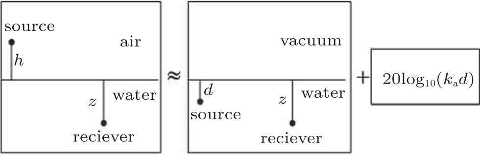 | Fig. 2. Modeling air-to-water transmission losses with standard numerical codes of underwater acoustics. |
The wavenumber integration approach is basically a numerical implementation of the integral transform technique for horizontally stratified medium. As this approach makes the least approximation, it can be used to obtain a benchmark result. According to the wavenumber integration approach, Schmit[16] developed a computer program referred to as OASES, which can be used to predict the air-to-water transmission.
One of the problems in the study of the air-to-water sound transmission is the rapidly moving airborne source. A moving source in free space results in a frequency Doppler shift. In a stratified ocean, because of effects such as refraction, boundary reflection, and the coherent summation of multiple arrivals at a receiver, moving source problems are more complicated. Clark et al.[17] and Jacyna and Jacobson[18] studied the effect of a moving source on the total acoustic field at a fixed receiver in a deep ocean with the ray theory in 1976 and 1977, respectively. Guthrie et al.[19] and Hawker[20] presented the acoustic field of a horizontally stratified ocean generated by a monochromatic point source moving slowly with constant horizontal velocity in terms of the normal-mode theory in 1974 and 1979, respectively. When the source speed is much smaller than the mode group velocity, Hawker[20] presented a method of achieving a stationary phase which is widely used in matched-field localization. In 1994, Lim and Ozard[21,22] obtained the acoustic field for a source moving with an arbitrary but small horizontal velocity by expressing the field as a sum of modes in terms of retarded times for the range-independent environment and the weakly range-dependent environment. In 1994, Schmidt and Kuperman[23] derived a spectral formulation of the Doppler-shifted field in a stratified waveguide by combining both source and receiver motion, and presented a more complete formulation of the Doppler effect than earlier modal formulation. In 2006, Buckingham and Giddens[24] developed a theory for the acoustic field in a three-layer waveguide (atmosphere, shallow ocean and sediment) based on the wavenumber integral. The unaccelerated source, such as a line source and a point source, moved horizontally in the atmosphere.
If an airborne source moves with a higher speed, the methods mentioned above are no longer applicable. In 1994, Kazandjian and Leviandier[25] presented a normal-mode theory for evaluating the acoustic pressure field generated by a uniformly moving airborne source, but this method costs a large amount of computation time. In 2004, Lv and Wu[26] presented an approach based on the Doppler frequency of a virtual source determined by the ray theory, and combined it with normal mode theory. They obtained a more accurate stationary phase point than Hawker’s solution for an airborne source moving at a high speed. Li[27] presented a modal expression for the acoustic pressure in a stratified waveguide generated by a moving airborne source in 2007, and this modal has some advantages of simple formula, definite physical meaning and easy implementation. In 2007, Zhang[28] developed a fast field program (FFP) to calculate the shallow water acoustic field generated by an airborne source, and this program has been extended to treat the elastic bottom environment and moving medium. With this model, the effects of the wind speed profile, the sound speed profile and the airborne source height together with the lateral wave are studied. He pointed out that the wind speed profile and the sound speed profile in air have a very significant effect on the sound propagation in air but a little effect on the transmitted sound under water. When the depth of the shallow water is much larger than the wavelength of sound, the lateral wave is greatly affected by the wind speed profile and sound speed profile. For the rapidly moving airborne source, he developed a two-dimensional wavenumber integration model which can be approximated by a one dimensional wavenumber integration model at the far field and studied the acoustic field in deep water and shallow water. In deep water, both the amplitude and the frequency of the received signal change with time. In shallow water, the amplitude of the received signal fluctuates quickly, the Doppler shift is evident, and the spectrum broadening is significant. For the lateral wave, its Doppler frequency shift is consistent with that of the signal in the air, and is much larger than that for the refracted wave.
Another problem in the study of the air-to-water sound transmission is the rough interface between the air and the water. In the real ocean, the sea surface is randomly rough, and the sound in air refracting into water will be random too. The rough sea surface also induces both the incident angle and the insonifying cone to change.
In 1972, Medwin and Hagy,[29] and Medwin et al.[30] formulated the transmission problem for a randomly rough interface between two dissimilar fluids, based on the Kirchhoff-Helmholtz integral. They pointed out that as the roughness increases, the coherent transmission term decreases while the incoherent term increases. However, there is a great difference in the mean square transmitted pressure between the experimental value and the theoretical value. In 1976, Meecham[31] studied the air-to-water sound transmission with a rough ocean surface, based on the high-frequency approximation. As the surface roughness increases, the mean square transmitted pressure at a small grazing angle increases evidently, and the enhancement reaches up to 10 dB. In 1976, Lubard and Hurdle[32] conducted an experiment and pointed out that the received energy increases with source frequency and ocean roughness increasing. Kuperman and Schmit[33–36] presented a self-consistent perturbation approach to treat scattering at rough interfaces in stratified fluid-elastic media, and a series of researches was published in 1976, 1989, and 1995. In 2003, Yan and Zhang[37] studied the air-to-water sound transmission in shallow water by using the BDRM method and they also studied the effect of a randomly rough boundary on the sound field by the coupling normal-mode method. The comparison with the field of a smooth sea surface shows that in a low wind speed scenario, the rough boundary slightly influences the mean field as well as the mean square field; whereas, in the strong wind case, the mean field decreases while the mean square field increases. This method can be used in the cases of high wind-speed and frequency, but it requires a huge calculation time, so the statistical result cannot be obtained easily.
In 2014, Zhang and Peng[38] analyzed the effects of rough interface on the air-to-water sound transmission in a horizontally stratified environment as shown in Fig.
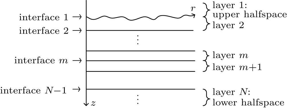 | Fig. 3. Horizontally stratified environment. |
Assuming that the interface at depth zi, separating the layers i and i + 1, is not smooth, but randomly rough with an elevation γ(

After some algebraic operations, the Fourier spectrum of the scattered field and the mean field at interface i can be expressed as


They programmed the self-consistent perturbation approach by adding a calculation model which is used to calculate the scattered field to the internationally popular OAST. This model can reduce the calculation so it is easy to obtain the statistical result. The total underwater field generated by an airborne source is calculated by the model in the cases of different wind speeds and frequencies. Based on simulation results and their comparison with the transmission loss for the smooth boundary, the conclusions are obtained as follows: rough sea surface causes obvious fluctuations of the transmission losses of the total field and the fluctuation increases as the propagation range, frequency and wind speed increase; rough sea surface causes the mean field to decrease but the mean square field to increase, and the influences become larger as frequency and wind speed increase. Generally speaking, the greater wind speed and frequency show positive influences on the underwater field.
In the same year, according to the self-consistent perturbation approach, Zhang and Peng[39] analyzed the effect of the airborne source height on the air-to-water sound transmission in shallow water with a randomly rough sea surface. The numerical simulation results show that the fluctuation of the scattered field decreases as the source’s height increases. In contrast, the averaged energy of the total field is hardly influenced by the source’s height in the statistical sense.
Spatial correlation is an important characteristic and directly relevant to the detection of an underwater target and underwater communication. It is also a useful and efficient tool for predicting the performance of large acoustic arrays. Spatial correlation of the sound field generated by the waterborne source[40–43] has received lots of attention but there have been few researches about the airborne source. According to the normal-mode theory,[13,14] Zhang et al.[44] derived the mathematical expression for longitudinal horizontal correlation of an underwater sound field generated by an airborne source in 2016. They employed a simulation and the result demonstrates that the oscillation period of longitudinal horizontal correlation coefficient for a source in air is almost the same as that for a source in water. The mathematical expression derived gives a physical explanation for the longitudinal horizontal correlation’s oscillation structure.
Because of the huge difference in acoustic characteristic impedance between air and water, only a little energy generated by an airborne source could transmit into water. The detection and extraction of the signal received underwater are difficult. Therefore, there are few publications about experimental study of the air-to-water sound transmission.
In 1971, Young[8,9] conducted an experiment with a loudspeaker and measured the sound pressures in the air and the test pool at various distances from the loudspeaker rim, both with a microphone and with hydrophones. The sound pressure level showed that the loudspeaker can be replaced by an underwater virtual source. In Urick’s field experiment,[7] a Navy P3 Orion turboprop aircraft flew over hydrophones at two depths in deep water. They concluded that the ray theory contours and their far field approximation give a fair fit to the data obtained by this experiment. They also demonstrated that multiple reflections from the ocean boundaries significantly extend the duration of the aircraft’s noise signature in shallow water, compared with the corresponding deep water experiment. In 1976, Lubard and Hurdle[32] conducted an ocean experiment at the Naval Undersea Center (NUC) Oceanographic Tower west of San Diego, California, in 18-m-deep water. The airborne source is a high-intensity speaker, with an air microphone and an underwater vertical array 48 m away from the speaker receiving signals separately. They took a rough-ocean interface into account and presented the more transmission for the rough ocean than predicted for a smooth surface. The data also show that the underwater source strength increases with increasing source frequency and ocean roughness.
Relevant research progress has also been made in China. In 2003, Lv et al.[45] verified the feasibility of receiving underwater signals generated by a motionless airborne source. In 2008, in order to study the depth distribution of underwater sound intensity, Peng et al.[46] conducted an experiment with a high-power loudspeaker transmitting signals in air and receivers located in air and water. They gave the depth distribution of underwater sound intensity in different ranges near the airborne source. In the above experiments, the receiver was located near the source within 1 km. In 2011, Wang[47] conducted an experiment. A loudspeaker transmitting linear frequency modulation (LFM) signals in the air and an HLA placed on the seabed was used as the receiver. The distance between the loudspeaker and the HLA was increased up to 4 km. For this experiment, the transmission loss calculated by a wavenumber integration model is in good agreement with the experimental value as shown in Figs.
 | Fig. 4. Air-to-water sound transmission loss with frequency intervals of (a) 200 Hz–300 Hz and (b) 800 Hz–1000 Hz. |
In practice, inverse problems, such as geoacoustic inversions and source localizations have also received a great deal of attention. In 2010, Peng et al.[48] carried out an experiment for airborne source localization in the Yellow Sea. They used a high-power loudspeaker as an airborne source hung on a research ship floating near a horizontal line array (HLA) laid on the sea bottom measuring signals. They presented a matched bearing processing for estimating the airborne source localization, and the estimated location is in good agreement with the GPS measurements. Wang[47] proposed a source localization method based on the cross bearings and the beam forming which was tested by the experimental data. Shown in Refs. [24], [49]–[52] is a series of experiments with a single-engine, light aircraft flying over a sensor station in the shallow water. At the sensor station, a microphone above the surface monitored the sound in air, a vertical array detected the acoustic arrivals under water and a single, buried hydrophone received the signals in the sediment. They developed the Doppler-spectroscopy inversion technique for recovering the properties of the airborne source and the three environments, i.e., the atmosphere, the ocean and the sediment. Furthermore, they investigated properties of the sound field generated from a moving source in a viscous medium.
The experiment was conducted in 2011, just as the underwater field was generated by LFM signals. Both experimental and theoretical data were averaged over a certain bandwidth. Hence the transmission loss curves showed a relatively smooth change with distance, and these transmission loss curves are not suitable for studying the fine structure of air-to-water sound transmission loss.
In order to perform further analysis on the fine structure of air-to-water sound transmission in shallow water, the research on the underwater field generated by single-frequency signals is necessary. In 2013, the State Key Laboratory of Acoustics, Institute of Acoustics, Chinese Academy of Sciences conducted an air-to-water experiment in the South China Sea. Zhang et al.[53] studied the underwater sound field generated by a hooter hung on the research ship which transmitted 128-Hz multi-frequency signals based on data recorded in this experiment. An HLA with 256 hydrophones laid on the seabottom at a depth of 94 m was used as a receiver to receive the signal transmitted by the hooter 2.3 km-to-9.8 km away.
The data of this air-to-water experiment was analyzed to study the characteristics of the air-to-water sound propagation at frequencies 128 Hz and 256 Hz. Experimental and theoretical air-to-water sound transmission losses in a range of 0 km–10 km are presented in Fig.
 | Fig. 5. Comparison of air-to-water sound transmission loss between experimental and theoretical results, frequencies of the source: (a) 128 Hz and (b) 256 Hz. |
Based on data recorded in the experiment mentioned above, Zhang et al.[44] studied longitudinal horizontal correlation coefficients of an underwater sound field generated by an airborne source at different distances with a frequency of 128 Hz for the first time. The results of sea trials in four ranges are shown in Figs.
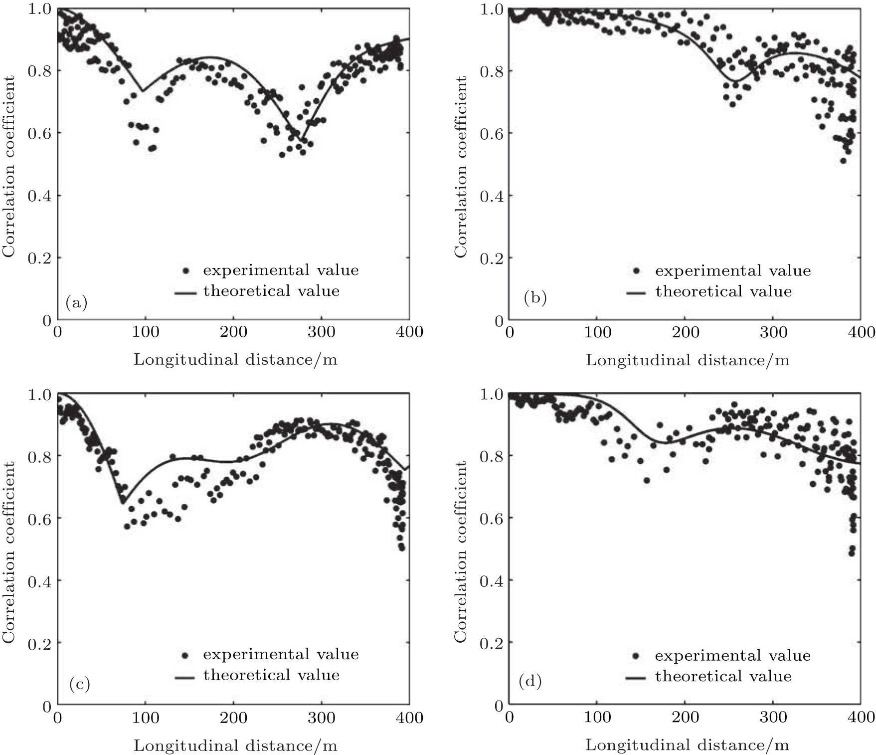 | Fig. 6. Comparisons of air-to-water sound transmission loss between experimental and theoretical results, with the distances between the research ship and the underwater horizontal line array being (a) 4.47 km, (b) 6.51 km, (c) 7.49 km, and (d) 9.47 km. |
In this paper, we review the theoretical and experimental research progress in the air-to-water sound transmission.
In theory, the first topic is to use four classical numerical methods to study the underwater sound field created by an airborne source, i.e., the ray theory, the wave solution, the normal-mode theory, and the wavenumber integration approach. Then, two special cases are presented: one is a rapidly moving airborne source or a moving medium, and the other is the rough interface between the air and the water. For the rough interface, this part offers the details of the self-consistent perturbation approach. At the end of this part the spatial correlation of the sound field generated by an airborne source is described based on the normal-mode theory.
In the experiment, firstly, we briefly introduce several influential experiments on the air-to-water sound transmission. Different kinds of airborne sources are used to study depth and range distributions of the underwater sound field in near-field and far-field. In terms of inverse problems, a Doppler-spectroscopy inversion technique for recovering properties of the environments and the airborne source and a matched bearing processing for estimating the airborne source localization are developed. Secondly, an experiment conducted in the South China Sea in 2013 with 128-Hz multi-frequency transmitted signals is discussed. Based on recorded data, experimental air-to-water sound transmission losses at frequencies 128-Hz and 256 Hz in a range of 2.3 km–9.8 km are in good agreement with theoretical results calculated by the wavenumber integration approach. The longitudinal horizontal correlation coefficients of an underwater sound field generated by an airborne source at different distances have the evident oscillatory behaviors, and the experimental values accord with the theoretical values.
| 1 | |
| 2 | |
| 3 | |
| 4 | |
| 5 | |
| 6 | |
| 7 | |
| 8 | |
| 9 | |
| 10 | |
| 11 | |
| 12 | |
| 13 | |
| 14 | |
| 15 | |
| 16 | |
| 17 | |
| 18 | |
| 19 | |
| 20 | |
| 21 | |
| 22 | |
| 23 | |
| 24 | |
| 25 | |
| 26 | |
| 27 | |
| 28 | |
| 29 | |
| 30 | |
| 31 | |
| 32 | |
| 33 | |
| 34 | |
| 35 | |
| 36 | |
| 37 | |
| 38 | |
| 39 | |
| 40 | |
| 41 | |
| 42 | |
| 43 | |
| 44 | |
| 45 | |
| 46 | |
| 47 | |
| 48 | |
| 49 | |
| 50 | |
| 51 | |
| 52 | |
| 53 |