

An efficient calibration method for SQUID measurement system using three orthogonal Helmholtz coils
[Li Hua1, 2, Zhang Shu-Lin1, †,  , Zhang Chao-Xiang1, Kong Xiang-Yan1, Xie Xiao-Ming1]
, Zhang Chao-Xiang1, Kong Xiang-Yan1, Xie Xiao-Ming1]
|
|


† Corresponding author. E-mail:
Project supported by the “Strategic Priority Research Program (B)” of the Chinese Academy of Sciences (Grant No. XDB04020200) and the Shanghai Municipal Science and Technology Commission Project, China (Grant No. 15DZ1940902).
For a practical superconducting quantum interference device (SQUID) based measurement system, the Tesla/volt coefficient must be accurately calibrated. In this paper, we propose a highly efficient method of calibrating a SQUID magnetometer system using three orthogonal Helmholtz coils. The Tesla/volt coefficient is regarded as the magnitude of a vector pointing to the normal direction of the pickup coil. By applying magnetic fields through a three-dimensional Helmholtz coil, the Tesla/volt coefficient can be directly calculated from magnetometer responses to the three orthogonally applied magnetic fields. Calibration with alternating current (AC) field is normally used for better signal-to-noise ratio in noisy urban environments and the results are compared with the direct current (DC) calibration to avoid possible effects due to eddy current. In our experiment, a calibration relative error of about 6.89 × 10⁻⁴ is obtained, and the error is mainly caused by the non-orthogonality of three axes of the Helmholtz coils. The method does not need precise alignment of the magnetometer inside the Helmholtz coil. It can be used for the multichannel magnetometer system calibration effectively and accurately.
As an extremely sensitive magnetic sensor, superconducting quantum interference devices (SQUIDs) are widely used for the very weak magnetic field measurements, such as magnetocardiography (MCG), fetal MCG, magnetoencephalography (MEG), etc.[1,2] SQUID is usually driven in flux-locked loop (FLL) read-out electronics, so that the output voltage varies linearly with the magnetic field which is scaled by the Tesla/volt coefficient. As a magnetic sensor, the sensing field magnitude should be precisely known from the voltage output of the SQUID channel. Therefore, the Tesla/volt coefficient of the SQUID system is very important and must be accurately calibrated, especially for a multichannel system.
In order to calibrate a multichannel magnetometer system, two kinds of methods were previously studied. A most traditional method used the single Helmholtz coils. A uniform field was imposed right on the magnetometer and the corresponding voltage output was measured.[3–5] Although effective, the direction of the uniform field must be precisely along the normal direction of the SQUID pickup coil. The other method was based on the measurements of signals generated by many small calibration coils. The unknown sensor parameters, including the Tesla/volt coefficient, were numerically estimated by using complex algorithms.[6–10] Additionally, all of the calibration was performed under a certain AC frequency.
In this paper, we propose a simple and yet efficient calibration method for the SQUID magnetometer system by using three orthogonal Helmholtz coils. The Tesla/volt coefficient can be treated as the magnitude of a vector pointing to the normal direction of the magnetometer. Based on the orthogonal uniform field offered by the three-dimensional Helmholtz coil, the Tesla/volt coefficient can be directly calculated. In our experiment, calibration under different frequencies and the traditional single Helmholtz coils, is measured and compared.
The magnetometer relies on the integrated pickup coil that picks up the measuring field and couples it to the SQUID. The voltage response of the magnetometer is proportional to the flux passing through the pickup coil area, which can be expressed as:


Figure
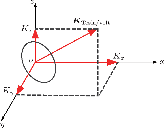 | Fig. 1. Calibration schematic for a SQUID magnetometer. |
By the orthogonal synthesis, the KTesla/volt can be expressed by

In this method, the calibration accuracy is directly influenced by two key parameters of the field uniformity and orthogonality of the three-dimensional Helmholtz coil. In order to evaluate the influences, digital simulation on these two parameters is first performed.
The field uniformity of one pair of Helmholtz coils is defined by the uniformity error Δε(x,y,z), which is expressed as
| Table 1. Values of uniformity error Δε of Helmholtz coil under different coil sizes. . |
For the field orthogonality of three-dimensional Helmholtz coil, a parameter of the orthogonality error Δε(α, β, γ) is used. Figure
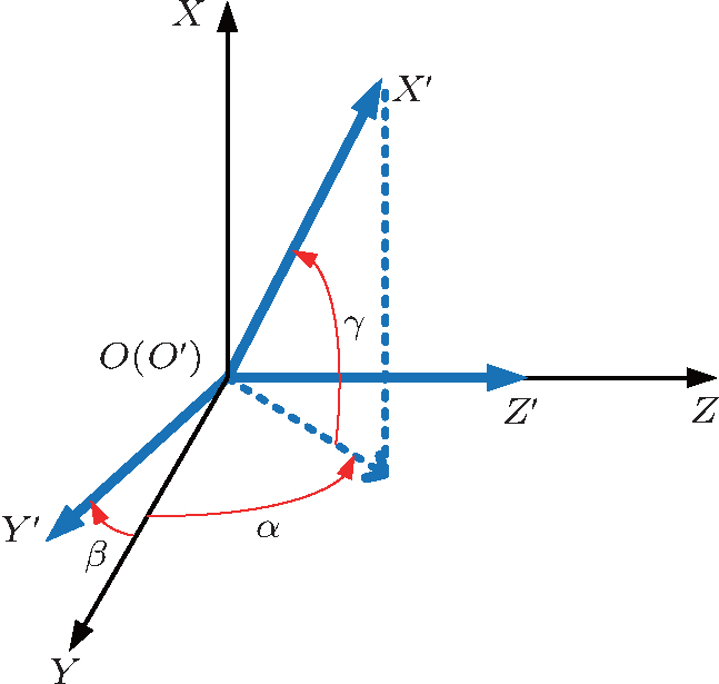 | Fig. 2. Relationship between orthogonal field |
The Δε(α,β,γ) corresponding to θ(α,β,γ) is defined as follows:

| Table 2. Calculated values of orthogonality error Δε(x,y,z). . |
Figure
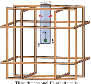
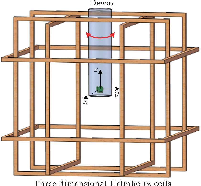 | Fig. 3. The calibration setup. |
Based on the experiment setup, the calibration under different applied frequencies from DC to several tens Hz are performed and compared with each other. Moreover, the independence of sensor orientation is also evaluated by rotating the cryostat along the XY-plane.
Calibration with AC field is normally used for better signal-to-noise ratio in noisy urban environments. In order to avoid possible effects due to eddy current, the AC calibration results are compared with DC calibration results. The calibration results under different frequencies from DC to 30 Hz are shown in Table
| Table 3. Several calibration results under different frequencies from DC to 30 Hz. . |
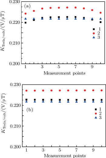
In order to illustrate the particularity with respect to the traditional method, comparison measurements are carried out. Figure
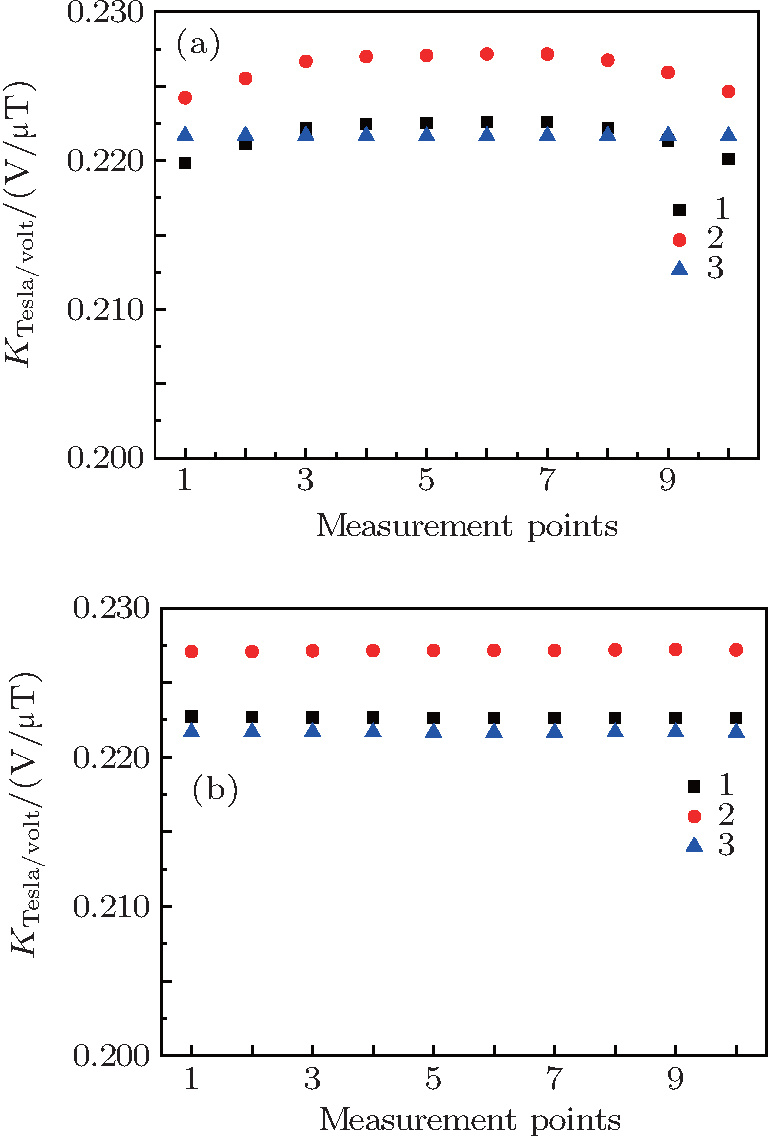 | Fig. 4. Comparison of measurement result between the traditional method (a) and our method (b): 1, 2, and 3 are three magnetometers; measurement points correspond to different rotation angles. |
We propose an efficient calibration method for the SQUID measurement systems using three orthogonal Helmholtz Coils. A calibration relative error of about 6.89 × 10⁻⁴ is achieved, which is mainly due to the non-orthogonal applied field. The results are shown to be independent of the applied frequency and sensor orientation. Without requiring the precise alignment of the magnetometer and complex algorithm, this method will be very convenient and effective for multichannel SQUID magnetometer system calibration.
| 1 | |
| 2 | |
| 3 | |
| 4 | |
| 5 | |
| 6 | |
| 7 | |
| 8 | |
| 9 | |
| 10 | |
| 11 | |
| 12 | |
| 13 |