Majorana fermions (MFs), with their antiparticles being themselves, have attracted lots of attention due to their development in the field of solid state physics in recent years.^[1] Their characteristics of non-Abelian statistics make possible their potential application in quantum computation.^[2–4] In order to experimentally observe the MFs, plenty of possible systems have been proposed. Among them, the fractional quantum Hall system,^[5,6] superconductor,^[7,8] and superfluid^[9,10] are believed to be the promising ways. Also, the existence of the MFs in a single quantum dot (QD), or in different QDs has been demonstrated in a system consisting of three QDs connected to two conventional superconductors by Deng et al.^[11] Moreover, it has been reported that Majorana bound states (MBSs) can be realized at each end of a semiconductor nanowire with strong spin-orbit coupling and Zeeman splitting when the nanowire is placed in proximity to an s-wave superconductor.^[12–15]

In spite of the achievements made in searching for the MBSs in solids, the exploration of the methods used to detect the existence of the MBSs is still a vexing question. Several groups have proposed many innovative ideas, such as the noise measurement,^[16–19] the resonant Andreev effect,^[20,21] and the fractional Josephson effect.^[22] Also, QD systems have been suggested as the possible candidates for detecting the MBSs. In 2011 Liu and Baranger found that the conductance through a QD system side-coupled to the end of a p-wave superconducting nanowire shows a sharp jump by a factor of 1/2 as the wire is driven through the topological phase transition, indicating the conductance may be viewed as a probe of the presence of the MBS.^[23] Then Cao et al. considered the transport through the QD under the finite bias voltage with particular attention paid to the Majorana's dynamic aspect, and found that a subtraction of the source and drain currents can expose the essential feature of the MFs.^[24] In 2013, Lee et al. considered the same setup yet with the QD in the Kondo regime, where they investigated the effect of the MBS on the Kondo physics, showing that the transmission through the QD provides an excellent way to detect the MBS in a much clearer way.^[25] Furthermore, the single QD setup side-coupled to the MBSs is generalized to the double QD case. In 2013 Wang et al. used the two QDs connected by an intermediate one-dimensional spin-orbit coupling nanowire to study the entanglement between the two QDs so as to expose the nonlocal quantum nature of the MBSs, which simultaneously provides further evidence for the existence of the MFs.^[26] Moreover, Zocher and Rosenow studied the charge transport through a topological superconductor with a pair of MBSs coupled to two leads via two QDs, which shows that the nonlocality of the MBSs opens the possibility of the crossed Andreev reflection (AR).^[27] Furthermore, based on the same setup, Liu et al. reported that the two nonlocal processes including the crossed AR and the electron tunneling (ET) can be directly controlled by gating the energy levels of the QDs.^[28] Also, Li et al.^[29] and Wang et al.^[30] performed the detailed investigation on the quantum transport of the double QD system coupled with the MBSs. Shang et al.^[31] investigated the electronic transport properties in an Aharonov–Bohm interferometer including two QDs coupled with Majorana fermions. These researches clearly demonstrate that many efforts have been made to detect or expose the nature of the MBSs by utilizing the interplays between the MBSs and the single QD or double.

Recently, the quantum transport through the QDs coupled with the MBSs are further extended to the multi-QD systems. Gong et al. studied the transport properties through a transverse T-shaped linear QD array with the MBS coupled to the terminal QD.^[32] It is shown that the existence of the Majorana zero mode completely modifies the electron transport properties of the QD structure. Furthermore, Jiang et al. studied the tunable quantum transport through the horizontal linear QD array with the MBS side-coupled to the QDs, indicating the feasibility to manipulate the current by means of the QD-MBS coupling.^[33] These researches are just a starting point of understanding how the MBSs affect the transport properties of the coupled QD systems. A further study on the QD transport properties in the presence of the MBSs is required so as to obtain some universal properties for comprehensively understanding the nature of the MBSs.

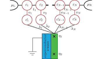
Motivated by the aforementioned works, in this paper we propose a serially coupled QDP chain system side-coupled with the MBSs as shown in Fig. 1. In this setup, sandwiched between leads L and R is the main chain including N QDs (QD-1, QD-2, …, QD-N) with each having a side-coupled QD (QD-1′, QD-2′, …, QD-N′, respectively) as its partner in each pair. The nearby MBSs realized by adhering one semiconductor nanowire with strong Rashba interactions to a grounded proximity-induced s-wave superconductor can be selectively coupled to one side QD or more. It should be emphasized that this setup is a nontrivial extension of the linear QD array due to the following reasons. (i) This is a renewed mixed QD structure, different from the isolated transverse or horizontal linear QD arrays, which is simultaneously characteristic of the transport properties of both the transverse and horizontal coupled QD arrays. It provides us with the opportunity of investigating the interplay of the effects of the two kinds of QD structures in the presence of the MBSs. (ii) The MBSs can be coupled to the QDP selectively, indicating that this setup is able to establish the multiple couplings between the MBSs and the QDP chain, which enables us to study the competition of the different couplings between the MBSs and the QDP. (iii) Due to the flexibility of the QDP, we can expose by using this QDP chain much deeper phenomena that are absent in the transverse and horizontal coupled QD arrays. We believe this study on the QDP chain with the side MBSs will present a much clearer picture of how the MBSs affect the quantum transport of the multiple QD structures.

In this paper, using the Green functions method we study the quantum transport properties through the double, triple, and quadruple QDP structures in the presence of the MBSs. First, we consider the conductance through the double QDP structure with the MBS side-coupled to QDP 1, 2, or both, respectively. It is shown that there exists a sharp AR-induced zero-bias conductance peak for the nonzero MBS-QDP coupling when the MBS is coupled to the far left QDP. Moreover, the MBS will make obvious influences on the competition between the ET and AR processes, which results in the splitting of the total conductance peaks of the isolated multi-QDPs. Then we study how the tunneling rate Γ^L affects the conductances of leads L and R to deeply understand the transport properties. As a generalization, we then numerically study the influences of the MBS in the triple and quadruple QDPs, which strongly supports the results obtained in the double QDPs. Finally we investigate the conductances of the single, double, triple, and quadruple QDP chains for the different inter-MBS couplings. A detailed comparison shows that the influence of the inter-MBS coupling in the multi-QDP chain is different from that in the single QDP one. These results should be instructive for understanding the influences of the interplay between the regular bound states and the MBSs on the quantum transport in such a kind of QD systems coupled with the MBSs.

The rest of the paper is organized as follows. In Section 2, the model Hamiltonian is presented, and the Green functions as well as the conductance formula are derived. In Section 3, we numerically investigate the conductance through the serially coupled multi-QDP chain. Finally, a brief conclusion is given in Section 4.

The serially coupled QDP chain structure that we considered here is schematically depicted in Fig. 1. The Hamiltonian of the entire system can be expressed as^[28–30]

Fig. 1.

	Figure Option ViewDownloadNew Window
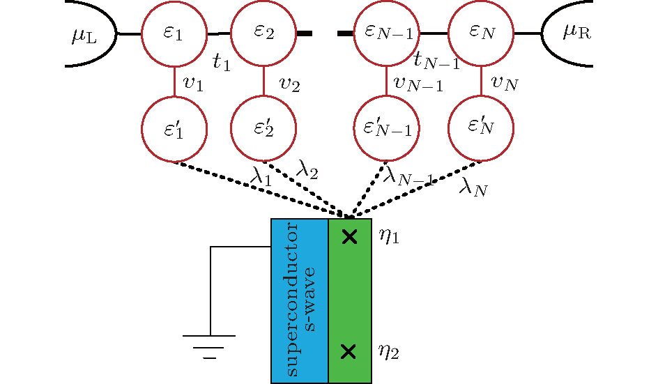
	Fig. 1. Schematic illustration of a serially coupled multi-QDP chain structure side-coupled with the MBSs by the MBS-QDP coupling λi (i = 1,2,…,N). The i-th QDP is composed of QD-i and QD-i′ with the energy levels εi and , respectively. The two MBSs are defined as η1 and η2, and the chemical potentials of the left and right leads are denoted by μL = EF + eV/2 and μR = EF − eV/2, respectively.

Here λ_i denotes the coupling between the side QD in the i-th QDP and the nearby MBS. Since there is a bias voltage eV applied between the two leads, we can write the chemical potentials in the left and right leads as μ_L = ε_F + eV/2 and μ_R = ε_F − eV/2, respectively. Hence, the different chemical potentials will lead to the current transport. In order to obtain the formula of the current following through the leads, the nonequilibrium Green function technique will be used.^[34–37] Finally, the current in the αth lead can be expressed as

Here is the electron’s (hole’s) Fermi distribution in lead α. is the ET coefficient, which describes the transmission probability from lead α to lead α′, and the transmission coefficient represents the local AR, in which G^R and G^A are the retarded and advanced Green functions in matrix form. For convenience, we replace the MF operators η₁ and η₂ by the regular fermion operators f and f^† via the relations and with {f, f^†} = 1. Thus, as usual, the retarded Green function is defined in the Nambu representation by G^R(x₁t₁,x₂t₂) ≡ − iθ(t₁ − t₂)⟨{Ψ(x₁t₁),Ψ^†(x₂t₂)}⟩ with the definitions Ψ(x₁t₁) ≡ (ϕ,ϕ^†)^T and Ψ^†(x₁t₁) ≡ (ϕ^†,ϕ) where ϕ can denote the fermion operators d_i, a_i, and f. By using the equation of motion method, the matrix form of the retarded Green function can be derived as^[32–36]

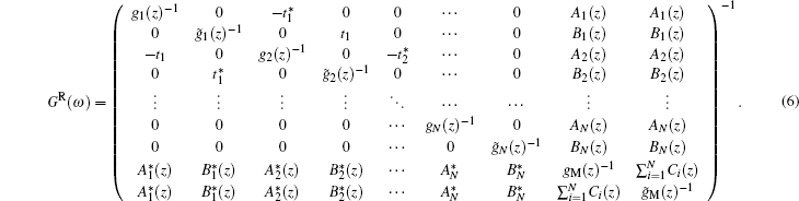
In the above equations, we have defined z = ω + i0⁺. Within the wide-band limit approximation, we will select in our calculation.

In this section, we will carry out the numerical investigation on the electron transport properties of the QDP chain structures coupled with the MBSs. Here the temperature T is chosen to be zero in the calculation, and the unit of the related parameters is selected to be 10⁻² meV as suggested in the previous work.^[27] Also, both the QD energy levels ε_i and , and the MBS-QDP coupling ε_M are taken to be 0 and all the interdot couplings v_i and t_i are chosen to be 1 except for those stated exceptionally.

3.1. Conductance with ε_M = 0

As a start, we study the quantum transport through the simplest double QDP chain composed of two QDPs in Fig. 2. For clarity, as the first step we consider the case that each QDP in the double QDP chain is separately coupled with the MBS. Figure 2(a) shows the conductance when the MBS is coupled with QDP 1 with λ₁ ≠ 0 and λ₂ = 0. For comparison, the conductance corresponding to λ_1,2 = 0 is also plotted by the lowest curve in Fig. 2(a). Clearly, a well-defined insulating band gap appears in the proximity of eV = 0, which is attributed to the Fano antiresonance. Also, four conductance peaks with G(eV) = 1e²/h are observed at eV = ±1.354 and eV = ± 3.190, which is determined by the resonance condition

and

with t₁ = v₁ = v₂ ≡ v and Γ^L = Γ^R ≡ Γ. In the double QDP case, according to the molecular energy levels

with of the serially coupled four QDs we can obtain the specific energy levels are ±1.236 and ±2.236. This indicates that the resonant transport is closely dependent on both the interdot couplings v and the QDP-lead couplings Γ, different from the single QDP case where the resonant peak positions are purely determined by the molecular energy levels ±t₁. Then we start to study the influences on the conductance G_L induced by the coupling λ₁ between QDP 1 and η₁. It can be seen in Fig. 2(a) that the nonzero λ₁ will induce a sharp conductance peak at eV = 0 in the band gap, and each of the original four conductance peaks at eV_1,2,3,4 is eventually split into two peaks. Also it is notable that the zero-bias conductance peak is able to amount to the conductance unit e²/h, which is different from the case of the single QDP side-coupled with the MBS where the zero-bias conductance is only e²/2h. To understand the conductances more clearly, we intend to extract from G_L the AR conductance G_A as shown by the dotted curves in Fig. 2(a). Clearly, in the case of λ₁ ≠ 0 there appears a sharp peak at eV = 0 in the conductance G_A curve, indicating that the central peak in the G_L curve is attributed to the AR process (see the curve with λ₁ = 0.2 which is aligned with the corresponding G_L curve in the band gap). Also, a pair of low side peaks are observed at eV_1,2, which is reasonable since the AR process is strengthened when the molecular energy level of the coupled QDs is aligned with the chemical potential μ_L of lead L. As λ₁ becomes large enough, another pair of side peaks at eV_3,4 emerges, further verifying that an AR conductance peak will appear whenever the QD molecular energy level is aligned with μ_L. Moreover, with increasing λ₁ the central peak becomes a little wider, and the two pairs of the side peaks become higher and wider. Meanwhile, the central peak is always pinned at eV = 0 with its height always equal to e²/h, the positions of the peaks at eV_1,2 are almost invariant, and the peaks at eV_3,4 move away from each other. This clearly shows that the zero-bias λ₁-induced conductance peak is robust against the coupling between the MBS and the QDP. Furthermore, by comparing G_A and G_L we can find that the AR process makes a great contribution to the central zero-bias conductance peak, the inner sub-peaks in the pair of side peaks at eV_1,2, and the outer sub-peaks in the pair of side peaks at eV_3,4. On the other hand, by a close inspection of the difference G_E ≡ G_L-G_A representing the ET conductance, we can find that each of the original four conductance peaks in G_E is split into two sub-peaks due to the coupling λ₁, indicating that the coupling λ₁ also has an obvious effect on the ET conductance G_E. As λ₁ increases, firstly the inner pair and then the outer pair of the peaks in G_A are enhanced, and simultaneously the overall ET conductance G_E is suppressed, which together induce the complex pattern of the total conductance, reflecting the competition between the normal ET process and the AR one.

Fig. 2.

	Figure Option ViewDownloadNew Window
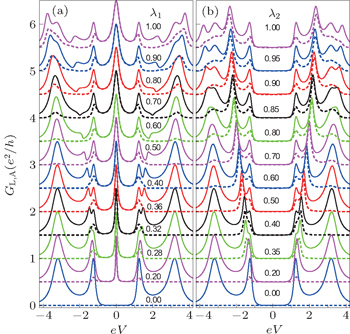
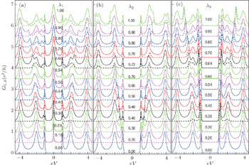
	Fig. 2. The total conductance GL (solid curves) and the corresponding AR conductance GA (dotted curves) in lead L through the double QDP chain versus the bias voltage eV between leads L and R when the MBS is coupled to QDP 1 (a) and QDP 2 (b). From bottom to top the curves are shifted up by 0.5e2/h in turn for clarity. The other parameters are taken to be ΓL,R = 0.5, t1 = 1, v1,2 = 1, and εM = 0.

Then we consider the quantum transport of the double QDP structure with the MBS coupled to QDP 2 by λ₂ in Fig. 2(b). First, different from the case of λ₁ ≠ 0 in Fig. 2(a), no zero-bias conductance peak appears in the band gap for any λ₂. Why? Actually, in the process of the electron transport from lead L to QD2 and vice versa the electron must pass through QDP 1. In this double QDP structure QDP 1 will prohibit the ET transport from lead L to QDP 2, and thus prevent the zero-bias conductance peak from appearing. Second, similar to that of λ₁ ≠ 0, every peak in both the inner and outer pairs of the conductance peaks corresponding to λ_1,2 = 0 is split into two sub-peaks with the increase of λ₂. To clearly see the competition between the ET and AR processes, we also plot the AR conductance by the dotted curves. As λ₂ increases, the AR conductance first shows one pair of low peaks at eV_1,2 (see the curve of λ₂ = 0.2), then one pair of discernable triple peaks (see the curve of λ₂ = 0.8), and finally the triple peaks are inclined to evolve into the wide peaks (see the curve of λ₂ = 1.0). Obviously, here the AR process mainly affects the outer sub-peaks in the pair of side peaks at eV_1,2, and the inner sub-peaks in the pair of side peaks at eV_3,4, which is different from or even opposite to the cases of λ₁ ≠ 0. Third, due to the competition between the ET and AR processes, the ET conductance G_E is suppressed and the AR one G_A is enhanced, as expected.

Next, in Fig. 3 we consider the conductance of the double QDP structure with the MBS coupled to both QDPs with λ_1,2 ≠ 0. Figure 3(a) shows the G_L ∼ eV curves for the different λ₁ in the case of λ₂ = 0.5. For comparison we first plot the G_L ∼ eV corresponding to λ₁ = 0, where the band gap is found in the proximity of eV = 0, and the AR process makes a great contribution to the outer sub-peaks in the pair of side peaks at eV_1,2. When λ₁ is tuned to be nonzero, e.g. 0.2, an AR conductance peak emerges at eV = 0 and the band gap disappears. As λ₁ increases, both the zero-bias peaks in G_A and G_L are becoming higher gradually with G_A < G_L, different from the cases of λ₂ = 0 with G_A = G_L shown in Fig. 2(a). This indicates that in the case λ₂ ≠ 0, the nonzero λ₁ not only induces the zero-bias AR conductance peak, but also opens the channel used for the electron to transport through QDP 1. At the same time, the original sharp AR conductance peaks at eV_1,2 are suppressed and eventually expunged, and two pairs of low AR peaks at eV_1,2 and eV_3,4 besides the zero-bias AR peak are inclined to emerge (see the curve with λ₁ = 1). This further demonstrates that there exists a competition in the AR conductance depending on the values of λ₁ and λ₂. To understand this competition more clearly, we plotted in Fig. 3(b) the AR conductance for different λ₂ in the case of λ₁ = 0.5. Obviously, the three characteristic AR conductance peaks induced purely by λ₁ (the dotted curve with λ₁ = 0.5) are seriously suppressed and new characteristic peaks are inclined to appear (the dotted curve with λ₂ = 1.0). This again verifies that the couplings λ₁ and λ₂ will induce a competition in the AR conductance, clearly unveiling the forming of the complex conductance pattern.

Fig. 3.

Figure Option ViewDownloadNew Window

Fig. 3. The total conductance GL (solid curves) and the corresponding AR conductance GA (dotted curves) in lead L through the double QDP chain versus the bias voltage eV when the MBS is simultaneously coupled to QDP 1 and QDP 2 for different λ1 with λ2 = 0.5 (a) and different λ2 with λ1 = 0.5 (b). From bottom to top the curves are shifted up by 0.5e2/h in turn for clarity. The other parameters are taken to be ΓL,R = 0.5, t1 = 1, v1,2 = 1, and εM = 0.

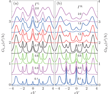
Now we turn to study the influences on the conductances G_L and G_R induced by the coupling Γ^L in Figs. 4(a) and 4(b), respectively, with λ_1,2 = 0.5 and Γ^R = 0.5. First, we can find in Fig. 4(a) that the conductances are uniformly strengthened with increasing Γ^L from 0 to Γ^R. This is because the increase of Γ^L will augment the tunneling probability of the electron from lead L to QDP 1, and thus augment the ET and AR processes simultaneously, which induces the increase of the conductance. However, when Γ^L > Γ^R, complex variation patterns of the conductance peaks appear instead of the uniform increase. With further increasing Γ^L, the central peak and the pair of peaks near eV = ±2 (type-I peaks) continue to become higher, while the pairs of peaks near eV = ±1.2 and eV = ±3.2 (type-II peaks) start to become lower. Obviously, it can be found that the AR conductance forms the peaks only at the positions of the type-I peaks and are almost negligibly small at those of the type-II peaks, indicating that the type-I peaks are contributed by both the ET and AR processes, while the type-II peaks are mainly by the ET process. As Γ^L increases, the AR induced peaks become high monotonically, while the ET induced peaks become first high and then become low after a big enough Γ^L. It is the different dependence on the Γ^L that produces the complex conductance patterns shown in Fig. 4(a). For comparison, we also show the corresponding conductance of lead R in Fig. 4(b). It is clear that the AR induced conductance peaks in lead R appear at the same positions of the type-I peaks, while their heights become low monotonically as Γ^L increases. Intuitively, this phenomena can be understood according to a simple three terminal setup, in which the electrons coming from two sources flow into a drain. Therefore, for a specific output in the drain, the increase of the conductance in one source must be accompanied by the decrease of that in the other. Moreover, we can find that the other conductance peaks appearing at the positions of the type-II peaks become low continuously as Γ^L increases. This should be understandable since the ET conductance in lead R is right equal to that in lead L, which induces the similar conductance patterns of the type-II peaks. Thus we can draw a conclusion that the couplings Γ^L,R not only affect the ET process between leads L and R, but also adjust the competition of the AR conductances in leads L and R.

Fig. 4.

	Figure Option ViewDownloadNew Window
	Fig. 4. The total conductance GL,R (solid curves) and the corresponding AR conductance GA (dotted curves) in leads L (a) and R (b) through the double QDP chain versus the bias voltage eV for different ΓL while ΓR = 0.5. From bottom to top the curves are shifted up by 0.5e2/h in turn for clarity. The other parameters are taken to be λ1,2 = 0.5, t1 = 1, v1,2 = 1, and εM = 0.

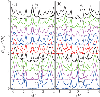
So as to understand the transport properties more completely and deeply, in the following we generalize the discussion from the double QDP system to the triple QDP system. Figures 5(a), 5(b), and 5(c) show the G_L ∼ eV curves of the triple QDP system when the MBS is coupled to QDP 1, QDP 2, and QDP 3, respectively. Obviously, for λ_1,2,3 = 0 three pairs of resonant transport conductance peaks are observed, as expected, indicating six molecular QD energy levels are formed. First, let us observe the curves in Fig. 5(a). As the coupling λ₁ increases, a zero-bias peak in the conductance G_L appears at eV = 0 and all the peaks corresponding to λ₁ = 0 are inclined to be split. By comparing the G_L and G_A curves, we can find that the zero-bias peak is mainly contributed by the AR process. Also, for a strong enough coupling λ₁, it can induce three pairs of AR conductance peaks near the molecular energy levels. Furthermore, we study the conductance pattern when the MBS is connected to QDP 2 and QDP 3 in Figs. 5(b) and 5(c), respectively. There are no zero-bias conductance peaks appearing in both cases, which should be reasonable since the transport channel from the lead L to QDP 2 is prohibited, as pointed out before. At the same time, the AR conductances show the different pairs of AR peaks depending on the specific couplings. It should be emphasized that, though the conductance patterns are different for the different couplings λ₁, λ₂, and λ₃, a uniform regularity of the ET conductances can still be found that the ET conductance peaks are inclined to be suppressed and split while the AR conductance is strengthened with the increasing of the MBS-QDP couplings.

Fig. 5.

	Figure Option ViewDownloadNew Window
	Fig. 5. The total conductance GL (solid curves) and the corresponding AR conductance GA (dotted curves) in lead L through the triple QDP chain versus the bias voltage eV when the MBS is coupled to QDP 1 (a), QDP 2 (b), and QDP 3 (c). From bottom to top the curves are shifted up by 0.5e2/h in turn for clarity. The other parameters are taken to be ΓL,R = 0.5, t1,2 = 1, v1,2,3 = 1, and εM = 0.

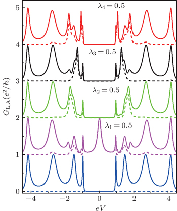
To provide a more convincing support to the conclusions drawn according to the double and triple QDP systems, we further show some typical conductance curves of the quadruple QDP system in Fig. 6. For comparison, we also plot the conductance of the isolated quadruple QDP with λ_1,2,3,4 = 0 where eight resonant ET conductance peaks are observed. Listed below are the most important influences of the MBS on the conductance. (i) Only when the MBS is coupled to QDP 1, there appears a zero-bias conductance peak which is purely induced by the AR process. (ii) Different conductance patterns of the quadruple QDP system are observed when the MBS is coupled to the different QDPs. (iii) As the MBS-QDP coupling increases, the conductance peaks of the isolated quadruple QDP system are inclined to be split, while the ET process will be suppressed and yet the AR process will be strengthened. All of these results are in agreement with the conclusions obtained from the double and triple QDP structures. Therefore it can be believed that the conclusion obtained in our study should be universal in this kind of QD systems in the presence of the MBSs.

Fig. 6.

Figure Option ViewDownloadNew Window

Fig. 6. The total conductance GL (solid curves) and the corresponding AR conductance GA (dotted curves) in lead L through the quadruple QDP chain versus the bias voltage eV. From bottom to top the curves are shifted up by e2/h in turn for clarity, which represent the conductances of the isolated QDP λ1,2,3,4 = 0, and those of the MBS coupled to QDP 1 (λ2,3,4 = 0), QDP 2 (λ1,3,4 = 0), QDP 3 (λ1,2,4 = 0), and QDP 4 (λ1,2,3 = 0), respectively. The other parameters are taken to be ΓL,R = 0.5, t1,2,3 = 1, v1,2,3,4 = 1, and εM = 0.

3.2. Conductance with ε_M ≠ 0

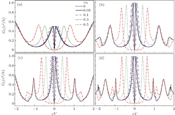
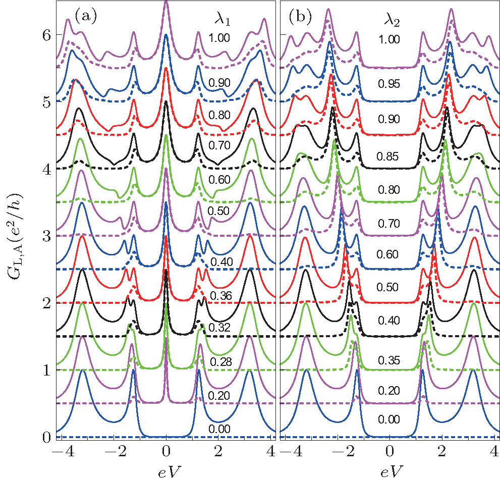
Finally, we intend to study the influences of the inter-MBS coupling ε_M between η₁ and η₂ on the conductances of the single, double, triple, and quadruple QDP systems in Fig. 7. Actually, when the MBS wire is selected to be enough short, the two MBSs will be coupled to each other and thus the inter-MBS coupling ε_M must be taken into account. For clarity, the MBS is on purpose coupled only to QDP 1 in the four cases shown in Fig. 7. For comparison, we first show the conductance G_L of the single QDP system for the different inter-MBS couplings in Fig. 7(a). It can be found that the nonzero ε_M can induce the appearance of the conductance dip in the zero-bias limit, similar to the results of Ref. [32]. That is to say, the nonzero ε_M will spit the zero-bias conductance peak with the height e²/2h into two sub-peaks, and as ε_M becomes larger, the two sub-peaks move away from each other and their heights become a little higher. Then we show the conductance of the double QDP chain in Fig. 7(b). We can clearly find that the most obvious variation of the conductance occurring in the proximity of eV = 0, where the AR-induced peak with the height e²/h is split into two sub-peaks. The complete transmission at eV = 0 becomes the complete reflection, indicating that this MBS-induced AR conductance peak is seriously affected by the coupling of the MBS with QDP 1. As ε_M becomes larger the two sub-peaks move away from each other and, however, their heights become lower, sharply different from the single QDP chain. Furthermore, we plot the conductance curves of the triple and quadruple QDP chains in Figs. 7(c) and 7(d), respectively. They show the similar phenomena to that of the double QDP chain. This clearly demonstrates that the inter-MBS coupling can make the zero-bias conductance peak split into two sub-peaks in the case of the multi-QDP chain, and the distance between the two sub-peaks becomes large and their heights become lower as ε_M increases, in contrast to that of the single QDP system. Also, by comparing Figs. 7(b)–7(d) we can find that the decay of the sub-peak heights of the multi-QDP structures becomes slower as the number of the QDPs increases. This should be an expectable result since the QDP is inclined to suppress the ET process from lead L to lead R, which is beneficial to enhancing the AR process in the lead L. This indicates that an increase of the number of the QDPs will strengthen the AR process further, leading to the slow decay of the sub-peaks as shown in Figs. 7(b)–7(d).

Fig. 7.

Figure Option ViewDownloadNew Window

Fig. 7. The conductances of the single (a), double (b), triple (c), and quadruple (d) QDP chains versus the bias voltage eV for the nonzero couplings εM between η1 and η2. In these structures, the MBS is only coupled to QDP 1 with λ1 = 0.5. The other parameters are chosen to be ΓL,R = 0.5 and v1,2,3,4 = 1. Also, t1,2,3 are equal to 1 and λ2,3,4 are equal to 0 if they exist in the corresponding geometries.

In conclusion, we have investigated the quantum transport properties of a serially coupled multi-QDP chain system side-coupled to the MBSs. It is shown that the nonzero MBS-QDP coupling will induce a sharp zero-bias conductance peak when the MBS is coupled to the far left QDP, which is absent when the MBS is coupled to the other QDPs. Besides the zero-bias conductance peak purely caused by the AR process, the MBS-QDP coupling can also induce other pairs of AR conductance peaks near the molecular QD energy levels and make obvious influences on the ET conductance. With the increase of the MBS-QDP coupling, the total conductance is inclined to be split with the ET conductance suppressed and the AR conductance enhanced, showing the competition between the ET and AR processes. Moreover, we study the influences of the tunneling rate Γ^L on the conductance of the multi-QDP chain. It is verified that Γ^L affects the conductances of leads L and R in different manners, clearly demonstrating that it can effectively adjust the competition between the AR and ET processes. Finally we consider the effect of the inter-MBS coupling on the conductances of the single, double, triple, and quadruple QDP systems. It is found that in the multi-QDP chains the inter-MBS coupling will split the zero-bias conductance peak with the height e²/h into two sub-peaks, which are moved away from each other as the inter-MBS coupling becomes stronger. Contrary to the single QDP structure with the sub-peaks becoming higher, the heights of the two sub-peaks are inclined to become lower. Furthermore, the decay of the conductance peaks with increasing ε_M becomes slow as the number of the QDPs becomes larger. We believe that this research should be greatly beneficial to understanding the quantum transport in this coupled QDP structure deeply and such a system may be viewed as a more promising candidate used to detect the existence of the MBSs.