A two-dimensional Lieb lattice,^[1] also called a line-centered square lattice, has attracted considerable research interest due to the specific properties induced by its topology. Each unit cell on the Lieb lattice contains three atoms (A, B, and C) (cf., Fig. 1(a)), and its energy spectrum is characterized by a three band structure with particle-hole symmetry, and a flat band touching two linearly dispersing intersecting bands at a single Dirac point (cf., Fig. 2(a)). The Lieb lattice is an interesting lattice model related to magnetism. Many theoretical studies on the flat-band ferromagnetism in the two-dimensional Lieb lattice have been performed,^[1–4] and recently the flat-band ferromagnetism in the multilayer or three-dimensional layered Lieb lattice was also investigated.^[5,6] Besides, the Lieb lattice exhibits other interesting properties, such as spectral and transport properties,^[7] nonlinear conical diffraction,^[8] superconducting transitions,^[9] spin fluctuations and superconducting pairing symmetries,^[10] magnon Hall effect,^[11] magnetic phase diagram,^[12] fractional Chern insulator phase,^[13] and Chern semimetals.^[14] Actually, several real materials can have their atoms arranged in the Lieb lattice. A most typical example is the CuO₂ planes of cuprate superconductors.^[15,16] Additionally, it is proposed that the Lieb lattice can be realized in different physical platforms, such as cold atoms in optical lattices^[17–19] and light propagation in photonic crystals.^[20,21] The bulk and edge transport phenomena in photonic Lieb lattices have been observed experimentally.^[21] Very recently, the first experiment realization of a dispersionless localized flat-band state in Lieb photonic lattices was independently reported by two groups.^[22,23]

Fig. 1.

Figure Option ViewDownloadNew Window

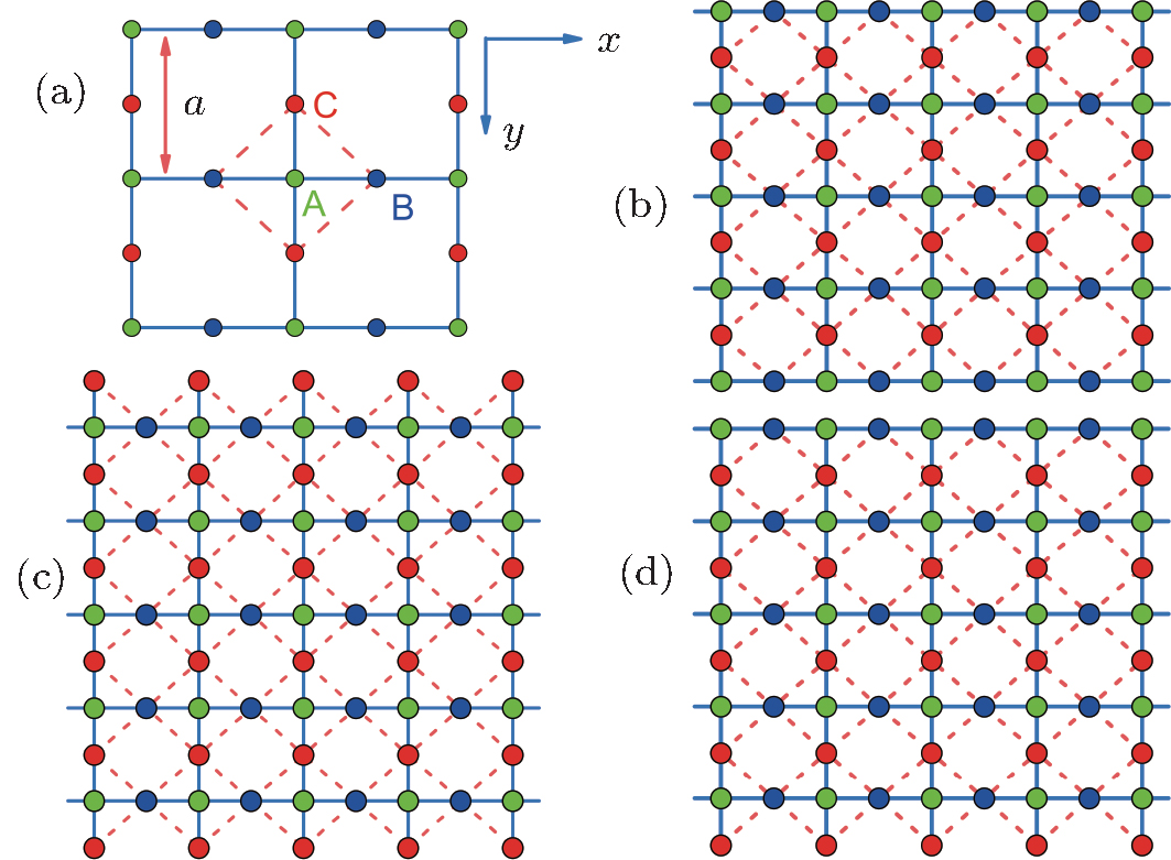
Fig. 1. (a) A two-dimensional Lieb lattice. The unit cell contains three atoms: A (green dots), B (blue dots), and C (red dots). The solid lines represent NN hopping, and the dashed lines represent the NNN hopping with ISO coupling. (b) Scheme of the strip lattice with the straight edges. Both sides (the upper and lower boundaries in the y-axis direction) of the lattice constitute A and B atoms. Here and hereafter, a periodic boundary condition is imposed along the x-axis direction. (c) Scheme of the strip lattice with the bearded edges, in which both sides of the lattice are terminated with C atoms. (d) Scheme of the strip lattice under the asymmetry boundary condition, in which one side is terminated with the straight edge and the other with the bearded edge.

Fig. 2.

	Figure Option ViewDownloadNew Window
	Fig. 2. The energy spectrum of the Lieb lattice. (a) The case without ISO coupling (λ = 0). Dirac cones appear and the three bands get in contact at k = (π,π). (b) The case with ISO coupling (λ ≠ 0). The gaps open between the flat band and the upper and lower dispersive bands.

On the other hand, quantum spin Hall (QSH) effects, also called two-dimensional topological insulators, and three-dimensional topological insulators have become immensely popular and active research fields in the condensed matter physics community.^[24,25] When the intrinsic spin–orbit (ISO) coupling is introduced to the Lieb lattice, a topologically nontrivial bulk gap is opened and it gives rise to the QSH effect characterized by two pairs of gapless helical edge states within the bulk gap.^[26] Recently, topological phase transitions driven by different parameters on the Lieb lattice have also been further investigated.^[19,27–30] It is noted that the finite size effect in topological insulators was firstly proposed in QSH states of HgTe quantum well, due to the fact the edge states on the two sides can couple together to produce a gap in the spectrum.^[31] Later, the finite size effect has also been predicted theoretically in three-dimensional (3D) topological insulator thin films.^[32–35] Moreover, the gap due to the finite size effect has been confirmed experimentally.^[36,37] It is proposed that the role of the finite size effect in topological insulators should be considered seriously in potential use of the topologically protected edge (surface) states in applications on the nanometer scale. Additionally, it was also found that the edge geometries of two-dimensional topological insulators have significant influences on the edge modes and the finite size effect of QSH states.^[38–43]

In this paper, we focus on the influence of the different edge geometries of the strip Lieb lattices on the finite size effect of helical edge state. Three kinds of edge geometries, i.e., straight, bearded and asymmetry edges (cf., Figs. 1(b)–1(d)), are investigated, respectively. Based on the tight-binding model, the spectrum and wave function of edge modes are derived analytically. For a strip Lieb lattice with two straight edges, the Dirac-like edge modes evolve from the Dirac-like bulk states without ISO coupling. Most significantly, the analytical results show that in this case the gapless Dirac-like spectrum remains unchanged with decreasing the width of the strip Lieb lattice, and no gap is opened in the edge band while the width of the strip model is comparable to the localization length of the edge modes. In sharp contrast to the HgTe quantum well discussed previously,^[31] for the strip Lieb lattice with the straight edges the finite size effect of QSH states vanishes. However, as opposed to the straight edges, for both the bearded and asymmetry edges, the energy gap induced by the finite size effect is still opened with decreasing the width of the strip. It is also demonstrated that the finite size gap decays exponentially with the sample width and varies non-monotonically with the amplitude of ISO coupling. Additionally, we illustrate the edge bands dispersion of the Lieb lattice can be controlled by applying an on-site potential to the outermost atoms.

This paper is organized as follows. In Section 2, we firstly review the main results on the spectra and the wave functions on the Lieb lattice in the momentum space. In Section 3, we discuss the edge modes under semi-infinite boundary conditions based on a tight-binding model of the Lieb lattice with straight and bearded edges, respectively. In Section 4, we investigate the edge modes on the Lieb lattice with the strip geometry. Three kinds of edge geometries, i.e., the straight, bearded and asymmetry edges, are considered, respectively. In Section 5, we demonstrate the controllability of the edge bands dispersion on the Lieb lattice. Finally, we give a summary in Section 6.

We start from the Hamiltonian of the tight-binding model for a two-dimensional Lieb lattice with ISO coupling^[26]

Now we apply a Fourier transformation to the real-space Hamiltonian (Eqs. (1)–(3)) (lattice constant a ≡ 1) to obtain the Hamiltonian in momentum space,

The eigenvalues of the Hamiltonian (5) are described by

For the case without ISO coupling (i.e., t ≠ 0 and λ = 0), the spectrum consists of three bands (per spin component), where the upper and lower bands touch the flat middle band via a cone-like dispersion at k = (π,π) (see Fig. 2(a)). From the wave function of the flat band , it is indicated that the flat band is composed only from orbitals of the types B and C atoms of the Lieb lattice without ISO coupling. However, when ISO coupling is considered (i.e., t ≠ 0 and λ ≠ 0), the zero-energy eigenfunction may also sit on the A-type sites. Furthermore, the ISO term opens two bulk energy gaps E_g = 4λ between the flat band and electron and hole branches at k = (π,π) (see Fig. 2(b)), respectively. Weeks and Franz have proposed that the gap induced by ISO coupling is characterized by the nontrivial Z₂ topological invariant υ = 1, and the Lieb lattice with ISO coupling is a typical model of two-dimensional topological insulators.^[26] Equivalently, an analytic calculation of the spin Chern number of the bulk state eigenvectors also demonstrates the occurrence of the QSH effect in the Lieb lattice when ISO coupling is included.^[19,27,28] By virtue of the bulk-boundary correspondence, there will be a pair of topologically protected helical gapless edge states along each edge in the lattice model with a strip geometry.

In the following, we will focus on the edge modes under different boundary geometries based on the analytical computation for a tight-binding model on the Lieb lattice.

In this section, we discuss the edge modes on the Lieb lattice with a semi-infinite geometry. Here a periodic boundary condition is imposed along the x-axis direction, and the initial open boundary of the half plane (along the y-axis direction) is assumed to locate at y = 0. Then a Fourier transformation is applied to the real-space along the x-axis direction, the momentum k_x as a good quantum number appears in the one-dimensional tight-binding Hamiltonian of the Lieb lattice.

3.1. The case with the straight edge

Firstly, we focus on the case of semi-infinite geometry with a straight edge. Here, we mention that in the y-axis direction the half plane begins with the type A and B sites (see the upper boundary in Fig. 1(b)). The corresponding Schrödinger equation for the spin-up part is given by

where

and with τ₀ = 2tc_x and τ_so = 2λs_x. Here we only consider the edge modes. The edge states are expected to be exponentially localized on the boundary, thus we use the following ansatz solution:^[44–46]

where ρ is a general complex number, and j is the index of the j-th lattice unit cell in the y-axis direction. For |ρ| < 1, the solution of Eq. (14) decreases exponentially with j. Thus the ansatz solution (14) can be used to describe the edge state localized on the boundary. Moreover, the results given by the ansatz solution (14) are consistent with those of numerical diagonalization. Then equation (12) can be reduced into the two equations as follows, an initial equation

and the inner one

with j = 2, 3, …, ∞.

By solving Eqs. (15) and (16), one can get the energy spectrum of spin-up edge state

and the corresponding eigenstate

with

It is indicated that the edge mode is composed only from orbitals of types A and B of the Lieb lattice with a straight edge.

In a similar manner, we can obtain another edge mode for spin-down, and the corresponding energy is given by

with

From Eqs. (17) and (20), it is found that the edge energy band is irrelevant to the amplitude of ISO coupling λ. The reason is that ISO coupling is introduced in NNN hopping (i.e., hopping between site C and site B), while the type C atom of the Lieb lattice does not contribute to the edge states (see Eqs. (18) and (21)).

3.2. The case with the bearded edge

Let us turn to the case of a different boundary geometry, the bearded edge. In the y-axis direction, the half plane begins with the C-type sites (see the upper boundary in Fig. 1(c)). Under the semi-infinite boundary condition, the corresponding Schrödinger equation for the spin-up part is given by

with

and . We assume an edge state solution as follows:

with |χ| < 1. Substituting Eq. (24) into Eq. (22), one can get two equations as follows:

By solving Eqs. (25) and (26), one finds that for the spin-up part there are two branches of edge modes with the energy bands

and the corresponding eigenstates

where

and

Two branches of edge modes given by Eq. (27) are plotted in blue and red dashed lines, respectively, in Fig. 3(a). Contrary to the case of the straight edge, for the case with the bearded edge the edge mode is composed from orbitals of the types A, B, and C of the Lieb lattice.

Likewise, two branches of the edge mode for the spin-down part are given by

with

Fig. 3.

Figure Option ViewDownloadNew Window

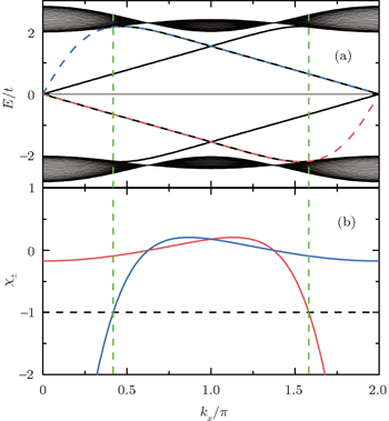
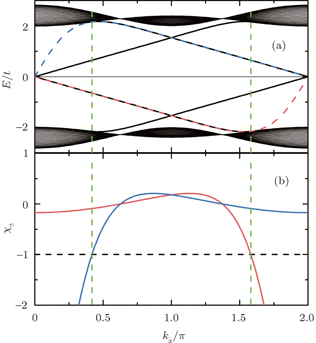
Fig. 3. (a) Energy spectrum obtained by numerical diagonalization of the tight-binding Hamiltonian for the spin-up part with λ = 0.6t and the number of unit cells n = 30 along the y-axis direction of the strip lattice with bearded edges. The blue and red dashed lines correspond to the energy given by Eq. (27), respectively. (b) The variations χ± with kx. The blue and red solid lines correspond to χ+ and χ−, respectively. Here, the green dashed lines locate at .

3.3. The characteristic parameter of the edge modes

The parameters ρ and χ (with |ρ|, |χ| <1) in Eqs. (14) and (24) characterize the localization scale of the edge modes. Defining , then l₀ denotes the localization length of the edge mode.

From Eq. (19), it is found that when k_x = 0 and 2π, |ρ| = 1. Thus, for the case with the straight edge, the edge mode merges into the bulk excitations at the center of the Brillouin zone. By solving |χ_±| = 1, one can obtain

here is the momentum where the edge states merge into the bulk states for the case with the bearded edge. In Fig. 3, are highlighted by green dashed lines. For , |χ₊| ⩾ 1, and for , |χ₋| ⩾ 1, therefore, the edge mode is absent.

For the case with the straight edge, the edge energy bands are irrelevant to the amplitude of ISO coupling λ, while the characteristic parameter ρ varies with λ. However, for the case with the bearded edge, both the edge energy bands and the characteristic parameters χ_± are dependent on λ. At k_x = π, ρ = ρ₀ = (2λ − t)/(2λ + t) and χ_± = χ₀ = (4λ² − t²)/(4λ² + t²). The variations of |ρ₀| and |χ₀| with λ are shown in Fig. 4. With the increase of λ from zero, |ρ₀| and |χ₀| decrease first up to zero at λ = 0.5t and then increase. It is indicated that the localization lengths of the edge modes vary non-monotonically with the amplitude of ISO coupling λ. At λ = 0.5t, |ρ₀| = |χ₀| = 0, that is, the edge states are completely localized on the outermost atoms. Notice that Wada et al. have theoretically studied the generic behavior of the localization length of the edge states in two-dimensional QSH systems.^[41] It was found that the minimum localization length corresponds to the inverse of the momentum-space width of edge-state dispersion. If the edge state extends almost over the whole Brillouin zone, the minimum localization length of the edge states is of the order of the lattice constant. On the Lieb lattice, for both the case with the straight edge and the case with the bearded edge, at λ = 0.5t (in this case the localization length is minimum when k_x = π) the edge states extend almost over the Brillouin zone, thus the minimum localization length of the edge states is as short as the lattice constant and the edge states in these two cases are localized on the outermost atoms. Additionally, from Fig. 4, it is shown that the localization length of the edge mode in the case with the straight edge is smaller than the case with the bearded edge for the same value of λ (except λ = 0.5t).

Fig. 4.

	Figure Option ViewDownloadNew Window
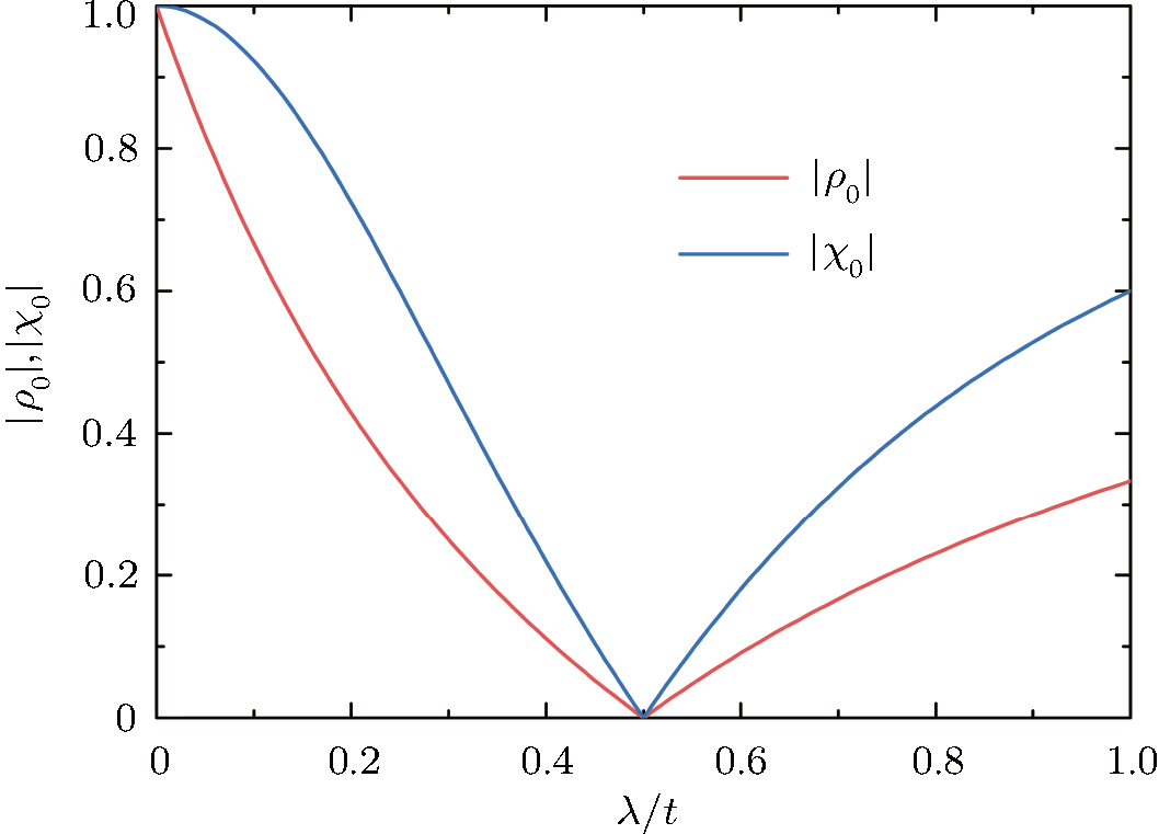
	Fig. 4. The variations of |ρ0| and |χ0| with λ. The red and blue lines correspond to |ρ0| and |χ0|, respectively.

In this section, we will investigate the edge modes on the Lieb lattice with the strip geometry. When the width of the strip model is comparable to the localization length of the edge modes, the finite size effect of QSH states has to be considered. Below, the finite size effect under three different kinds of boundary conditions, i.e., the straight, bearded and asymmetry edges, are examined, respectively.

4.1. The case with the straight edges

For the strip geometry with the straight edges, as shown in Fig. 1(b), both the upper and lower edges are composed by A- and B-type atoms, and a periodic boundary condition is still imposed along the x-axis direction as mentioned above. Considering a strip Lieb lattice with n unit cells along the y-axis direction, the total atom number is 3n − 1. A- and B-type atoms have the same atom number n, while the number of C-type atoms is n − 1.

We will first consider a simple case, which only contains three unit cells with eight atoms along the y-axis direction, then the eigenstate for the spin-up part is assumed as follows:

and the determinant of the secular equation for the tight-binding Hamiltonian is

with

and ε_a, t_a are given in Eq. (13). By solving F_s(3) = 0, we can get the eight eigenvalues

Here, we only write the wave functions corresponding to the two flat bands and the edge bands ,

with ρ_± = (τ_so∓t)/(τ_so±t). N_i (i = 1,2, 3, 4) is the normalization factor. When ISO coupling is considered, A-type atoms are involved in constituting the flat bands. The spectrum of the edge states is unaffected by the amplitude of ISO coupling λ, while the distribution of wave function varies with λ.

For the larger number of unit cells n (⩾3), the general eigenstates and the determinant of the secular equation for the spin-up part are written as follows:

and

We can derive the recursion formula for the determinant F_s(n),

with i = 3,4, …, n. G_s(i) and J_s(i) are the intermediate variables. The coefficients of the recursion formula are given by

and the initial values are

with and . Then we obtain the general expression of F_s(n),

where Q_± = α ± β, , and .

Letting F_s(n) = 0, it is easy to find and are always the solutions of the secular equation. The components of eigenstates corresponding to eigenenergy are obtained

Thus, are the energy spectra of edge modes for the spin-up part. The edge states corresponding to the spectra and localize at the upper and lower boundary of the strip geometry with the straight edges, respectively. It is emphasized that the edge spectrum in the strip geometry with the straight edges are the same as the case under semi-infinite boundary conditions with the straight edge (see Eq. (17)). In other words, in this case with two straight edges the gapless Dirac-like spectrum remains unchanged with decreasing the width of the strip Lieb lattice, and no gap is opened in the edge band. Generally, in QSH systems, the edge states on the two sides of a strip of finite width can couple together to open a gap in the edge energy spectrum. From Eq. (46), the components of eigenstates corresponding to the edge mode, it is shown that the wave functions of the two edge states localized at the upper and lower boundary do not couple together at the Dirac point, thus no gap is opened in the edge band with the strip width decreasing. Thus, it is concluded that the finite size effect of QSH states is absent on the Lieb lattice in the strip geometry with the straight edges. Such a finding is a new result, which is qualitatively distinct from the finite size effect on the HgTe quantum well discussed previously.^[31] Additionally, the edge modes are composed only from orbitals of the types A and B and irrelevant to C-type atoms, which is consistent with the result obtained under the semi-infinite boundary condition.

The degeneracy of the flat bands is n − 1, which is equal to the number of C-type atom along the y-axis direction on the Lieb lattice. The dispersive bulk energy spectra can be given by solving the following equation

where N = 1,2,…, n − 1. So the spectra of the dispersive bulk states have the following expression

We notice that for λ ⩾ t/2, at the momenta

the dispersive bulk energy spectra are (n −1)-fold degeneracy and can be given by

The energy spectrum and wave function distribution for the spin-up part are plotted in Fig. 5, obtained by numerical diagonalization of the tight-binding Hamiltonian of a strip lattice geometry. In fact, the above results given analytically are consistent with those of numerical diagonalization. In the absence of ISO coupling (i.e., λ = 0), it is shown in Fig. 5(a) that the gapless Dirac-like spectrum (±2t |cos (k_x/2)|) is intersected by the flat bands. By checking the wave function distribution of the Dirac-like spectrum (see the upper layer in Fig. 5(d)), it is found that this Dirac-like spectrum actually corresponds to the bulk state. Taking into account the ISO coupling (i.e., λ ≠ 0), the Dirac-like spectrum remain still unchanged (see Fig. 5(b)), but now it corresponds to the edge mode (see Fig. 5(d)). In Fig. 5(c), we plot the dependence of the spectrum on λ at k_x = π + 0.1, in which three straight lines appear: the green line corresponding to the flat bands and two red lines to the edge states. It is indicated that for a strip Lieb lattice with two straight edges, the ISO coupling induces the Dirac-like bulk states to localize at the edges to become the helical edge states with the same Dirac-like spectrum. It means that in this case with the straight edges the Dirac-like edge modes evolve from the Dirac-like bulk states without ISO coupling. We also notice that the conduction and valence bands near the flat bands are pushed up and down with the increase of λ, and all the conduction (valence) bulk states degenerate with E_c = 2.0025t (E_v = −2.0025t) at λ = 0.500626t (for k_x = π + 0.1), which can be obtained by Eqs. (49) and (50). For the case with the straight edges, the edge energy bands are irrelevant to the amplitude of ISO coupling λ, while the localization scale of the edge mode varies with λ. In Fig. 5(d), we plot the distribution of wave function corresponding to the Dirac-like spectrum with different amplitude of ISO coupling λ. The localization length of the edge mode varies non-monotonically with λ, which is consistent with the case under the semi-infinite boundary condition with the straight edge (see Fig. (4)).

Fig. 5.

Figure Option ViewDownloadNew Window

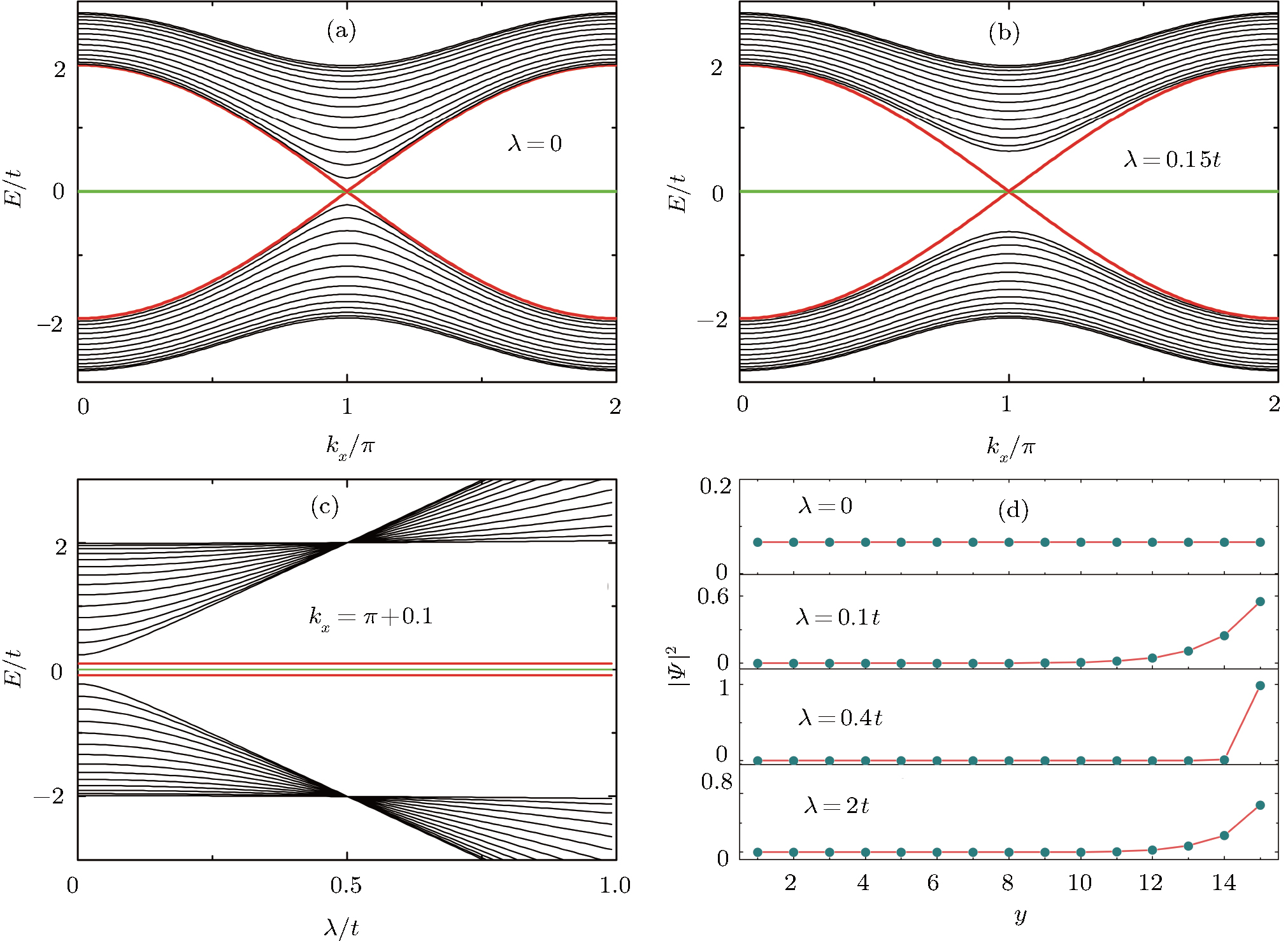
Fig. 5. Band structure and wave function distribution of H↑ in a strip geometry with the straight edges and the number of unit cells n = 15 along the y-axis direction. The green line corresponds to the flat bands. (a) The energy spectrum for the case without ISO coupling (λ = 0). The red lines correspond actually to bulk states. (b) The energy spectrum for the case with ISO coupling (λ = 0.15t). The red lines corresponds to edge states. (c) The variation of spectrum with λ for kx = π + 0.1. (d) The density distribution of wave function corresponding to the upper red line (E = 0.1t and kx = π + 0.1) in panel (c) for different values of λ.

4.2. The case with the bearded edges

Now we investigate the strip geometry with the bearded edges, which is schematized in Fig. 1(c). In this case, both the upper and lower edges are terminated with C-type atoms. Likewise, a periodic boundary condition along the x-axis direction is still considered. For a strip Lieb lattice with n unit cells along the y-axis direction, the total atom number is 3n + 1. A- and B-type atoms have the same atom number n, while the number of C-type atoms is n + 1.

Under the bearded boundary condition, the eigenstates and the determinant of the secular equation for the spin-up part are written as follows:

and

with

The recursion formula of the determinant F_b(n) can be derived as follows:

with i = 2,3,…, n, the coefficients

and the initial values

Then we can get the general expression of F_b(n)

with . When λ = 0, the expression of F_b(n) can be reduced into

Solving the secular equation F_b(n) = 0, we will obtain 3n + 1 eigenenergies of the Schrödinger equation for the spin-up part.

Firstly, we examine the case without ISO coupling (i.e., λ = 0). From the secular equation , we find (n + 1)-fold degenerate flat bands (E = 0) (the degeneracy n + 1 is equal to the number of C-type atom along the y-axis direction) and the dispersive bulk energy spectrum

with N = 1,2,…,n. At k_x = π, the conduction band bottom and the valence band top are given by

It is noted that a gap is opened between the flat band and the conduction band (or the valence band) (see Fig. 6(a)). When the width of strip Lieb lattice with the bearded edges is sufficiently large, i.e., in the limit of , then the gap closes.

Fig. 6.

Figure Option ViewDownloadNew Window

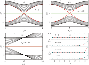
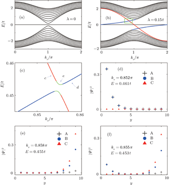
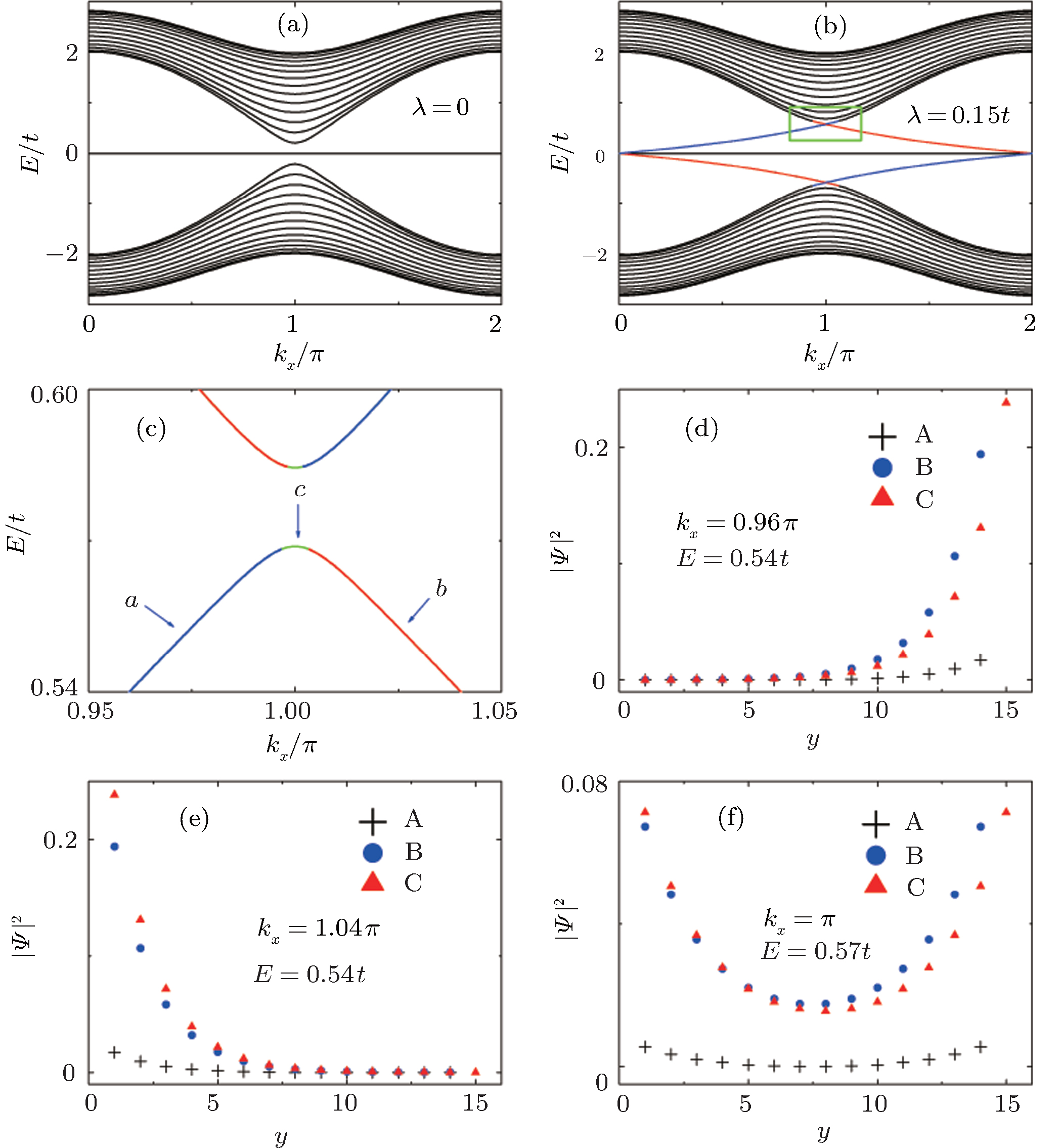
Fig. 6. Band structure and wave function distribution of H↑ in a strip geometry with the bearded edges and the number of unit cells n = 15 along the y-axis direction. (a) The energy spectrum for the case without ISO coupling (λ = 0). (b) The energy spectrum for the case with ISO coupling (λ = 0.15t). The red (blue) lines correspond to the edge modes whose wave function distribution are mainly located in the upper (lower) edge. (c) The larger version of the green rectangle in (b). The green lines correspond to the region in which two edge states on the upper and lower edges strongly couple together. (d), (e) and (f) are the wave function distribution corresponding to points a, b, and c shown in panel (c), respectively. Here, A, B, and C denote three types of atoms on the Lieb lattice presented in Fig. 1(a).

Now we consider the case with ISO coupling (i.e., λ ≠ 0). From the secular equation F_b(n) = 0, it is shown that the degeneracy of the flat bands is n − 1, but the other 2n + 1 eigenenergies of the Schrödinger equation for the spin-up part cannot be expressed analytically and only be obtained by numerically calculating the following equation

The energy spectrum and wave function distribution are shown in Fig. 6. As shown in Fig. 6(b), the edge modes appear within the bulk gap, but the Dirac points occur at k_x = 0 and k_x = 2π. The localization properties of the edge states are illustrated in Figs. 6(d) and 6(e). What we are concerned with is the finite size effect of helical edge states on the Lieb lattice with ISO coupling. In contrast to the case with the straight edges discussed above, the energy gap ΔE induced by the finite size effect can be observed on the strip Lieb lattice with the bearded edges (see Fig. 6(c). The finite-energy gap opens up at k_x = π due to the fact that the two sides edge states couple together presented by the wave function distribution in Fig. 6(f). It is emphasized that no edge state coupling happens at k_x = 0 and k_x = 2π (Dirac points), where the edge modes touch the flat bands. Additionally, from Figs. 6(d), 6(e), and 6(f), in contrast to the case with the straight edges, the edge modes are composed mainly from orbitals of the C- and B-type atoms, and the contribution of the A-type atom is far less than that of C- or B-type atom.

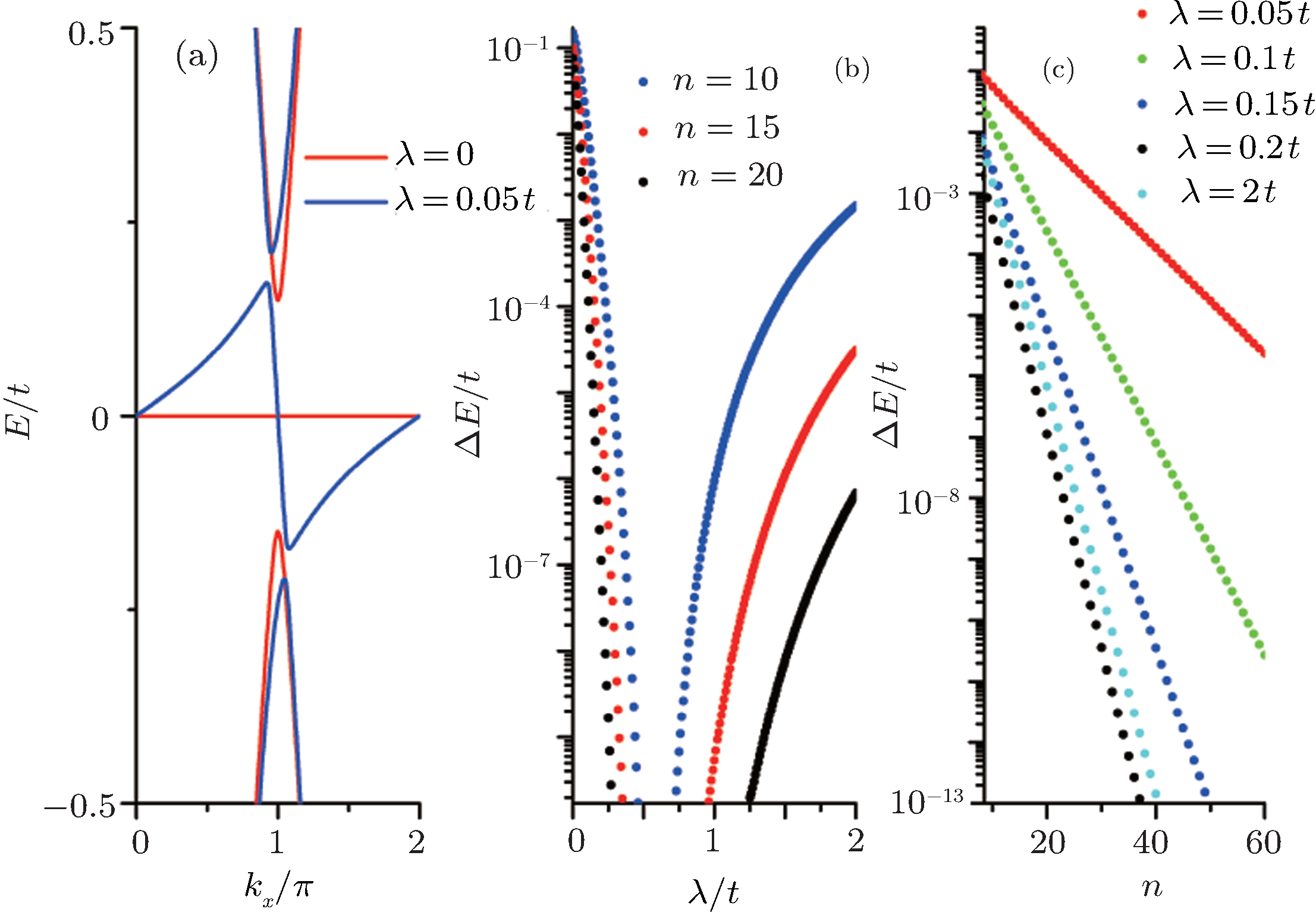
As mentioned above, for the strip Lieb lattice with the bearded edges, one of the key features for the solution of a finite width is the gap ΔE opening for the energy dispersion of the edge state. If n/l₀ ≫ 1, we can expand Eq. (61) at

where is given by Eq. (27) (with k_x = π), thus it can be found that a finite-energy gap is approximately

The inclusion of ISO coupling makes the degeneracy of the flat bands for the spin-up (or spin-down) part decrease from n + 1 to n − 1. It is indicated that two sides edge modes for spin-up (or spin-down) on the strip Lieb lattice with the bearded edges may evolve from two flat bands without ISO coupling. In Fig. 7(a), we plot a part of the spectrum of the edge states under the bearded boundary condition with n = 15 for different λ values. The variations of the energy gap ΔE induced by the finite size effect with λ for different n are plotted in Fig. 7(b) obtained by numerical diagonalization of the tight-binding Hamiltonian for the spin-up part. The non-monotonic variation of the gap ΔE with λ observed in Fig. 7(b) is due to the fact that the localization lengths of the edge modes vary non-monotonically with the amplitude of ISO coupling λ (see Fig. 4). In particular, for λ = 0.5t, the gap ΔE vanishes since in this case the distribution of the edge modes only locates at the outermost atoms. From Fig. 7(c), in which the variations of the gap ΔE with n for different λ are shown, it is found that the finite size gap ΔE decays exponentially with the sample width. It can be checked that the results given by Eq. (63) are approximately consistent with those obtained by numerical diagonalization if the condition n/l₀ ≫ 1 is satisfied.

Fig. 7.

	Figure Option ViewDownloadNew Window
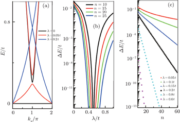
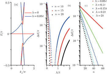
	Fig. 7. (a) Energy spectrum of edge states under bearded boundary condition with n = 15 for λ = 0, 0.05t, and 0.2t. (b) The variation of the gap ΔE with λ for different n. (c) The variation of the gap ΔE with n for different λ.

4.3. The case with the asymmetry edges

We proceed to study the strip geometry with the asymmetry edges. In the case with the asymmetry edges, it is assumed that the upper and lower edges of a strip Lieb lattice are the straight and bearded edge (see Fig. 1(d)), respectively. A, B, and C have the same atom number n and the total atom number is 3n for a strip geometry with n unit cells along the y-axis direction.

Under the asymmetry boundary condition, the eigenstates and the determinant of the secular equation for the spin-up part are written as follows:

and

The recursion formula of the determinant F_a(n) can be derived as follows:

with i = 2,3,…,n. The coefficients γ_ij of the recursion formula are given by Eq. (43), and initial values are

Then we can get the general expression of F_a(n),

with P = E³ − Eτ₀² + 4τ₀τ_sot. When λ = 0, the expression of F_a(n) can be reduced into

When ISO coupling is neglected (i.e., λ = 0), by solving the secular equation , we find n-fold degenerate flat bands (E = 0) and the dispersive bulk energy spectrum

with N = 1,2,…,n. At k_x = π, a gap opens up between the flat band and the conduction band (or the valence band top) (see Fig. 8(a)). Likewise, in the limit of n → ∞, the gap closes.

Fig. 8.

Figure Option ViewDownloadNew Window

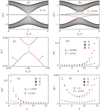
Fig. 8. Band structure and wave function distribution of H↑ in a strip geometry with the asymmetry edges and the number of unit cells n = 10 along the y-axis direction. (a) The energy spectrum for the case without ISO coupling (λ = 0). (b) The energy spectrum for the case with ISO coupling (λ = 0.15t). The red (blue) lines correspond to the edge modes whose wave function distribution are mainly located in the upper (lower) edge. (c) The larger version of the green rectangle in (b). The green lines correspond to the region in which two edge states on the upper and lower edges strongly couple together. Panels (d), (e), and (f) are the wave function distribution corresponding to points c, d, and e shown in panel (c), respectively. Here, A, B, and C denote three types of atoms on the Lieb lattice presented in Fig. 1(a).

Fig. 9.

	Figure Option ViewDownloadNew Window
	Fig. 9. (a) Energy spectrum of edge states under asymmetry boundary condition with n = 10 for λ = 0 and 0.05t. (b) The variation of the finite size energy gap ΔE with λ for different n. (c) The variation of the finite size energy gap ΔE with n for different λ.

When ISO coupling is considered on the Lieb lattice with a strip geometry (i.e., λ ≠ 0), the eigenenergies of the Schrödinger equation for the spin-up part can be obtained by solving the secular equation F_b(n) = 0. From Eq. (68), we can get (n − 1) -fold degenerate flat bands, and the other 2n + 1 solutions of the secular equation can be obtained by numerically calculating the following equation

We plot the energy spectrum and wave function distribution for the spin-up part under the asymmetry boundary condition in Fig. 8. From Fig. 8(b), the edge modes appearing within the bulk gap are observed. Since the two boundaries of the strip lattice are not equivalent, the edge states are not degenerate.^[26] The red line corresponds to the edge mode localized at the straight (upper) edge, and the blue line to the edge mode localized at the bearded (lower) edge. The localization properties of the edge states are illustrated in Figs. 8(d) and 8(e). The wave function distribution shown in Fig. 8(f) indicates that the two sides (upper and lower edges) edge states couple together at point e in Fig. 8(c), thus the energy gap ΔE induced by the finite size effect also opens in the edge energy spectrum under the asymmetry boundary condition. In contrast to the case with the bearded edges considered above, in the case with asymmetry edges the energy gap of the edge states will generically open at other finite k_x rather than at k_x = π. In Fig. 9(a), we plot a part of the spectrum of the edge states under the asymmetry boundary condition with n = 10. The non-monotonic variations of the finite size energy gap ΔE with λ for different n are plotted in Fig. 9(b) obtained by numerical diagonalization of the tight-binding Hamiltonian for the spin-up part. From Fig. 9(c), it is also found that the finite size gap ΔE decays exponentially with the sample width. Compared with the case under the bearded boundary condition, the finite size gap in the strip lattice with asymmetry edges has a faster decay rate with increasing sample width for the same the amplitude of ISO coupling λ.

From the above discussion, it is shown that the edge states on the strip Lieb lattice with the straight edges have distinct bands dispersion from the case with the bearded edges. For the straight edge, if we take away the outermost A- and B-type atoms, that is actually the bearded edge. Identically, the bearded edge turns into the straight edge when the outermost C atoms are taken away. The edge spectra of the Lieb lattice can be controlled by applying an on-site potential U to the outermost atoms.^[47] As an example, we consider the case with λ = 0.5t. It is noted that for the case with λ = 0.5t, the edge states near k_x = π are almost completely localized on the outermost atoms (cf., Fig. 4).

Firstly, we take the lattice with the bearded edges to demonstrate this controllability. The on-site energy U is applied on the outermost C-type atoms and is tuned to different values from 0 to 100t. Here, the energy spectrum is obtained by numerical diagonalization of tight-binding Hamiltonian (1) with an on-site energy U. For clarity, in Fig. 10 only the edge modes corresponding to the edge states for spin-up and spin-down localized near the upper boundary are shown. When U increases, the edge bands dispersions lift upward. When U = 1t, the upper cross point of the edge bands for spin-up and spin-down merges into the bulk conduction band at k_x = π. With further increase of U, the edge bands also appears on the top of the bulk conduction band. At sufficiently large positive on-site potential U, the outermost C-type atoms on the Lieb lattice with the bearded edge are effectively decoupled from neighboring A- and B-type atoms, and the Lieb lattice effectively terminates with the straight edge. To see Fig. 10(f), when U = 100t, the edge band within the bulk gap is consistent with the case with the straight edge.

Next, we focus on the lattice with the straight edges, then the on-site energy U is applied on the outermost A- and B-type atoms. The controlling of the edge bands dispersion by U is shown in Fig. 11. Likewise, when U increases, the edge bands dispersions lift upward. Meantime, new edge bands peel off from the bulk conduction, valance and flat bands, respectively. With further increase of U, anticrossing of the edge bands with the same spin occurs (cf., Fig. 11(d)). When the positive on-site potential U is sufficiently large, the edge band within the bulk gap is consistent with the case with the beard edge (cf., Fig. 11(f)), since the outermost A- and B-type atoms on the Lieb lattice with the straight edge are effectively decoupled from neighboring C-type atoms, and the Lieb lattice effectively terminates with the bearded edge.

Fig. 10.

Figure Option ViewDownloadNew Window

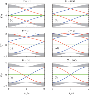
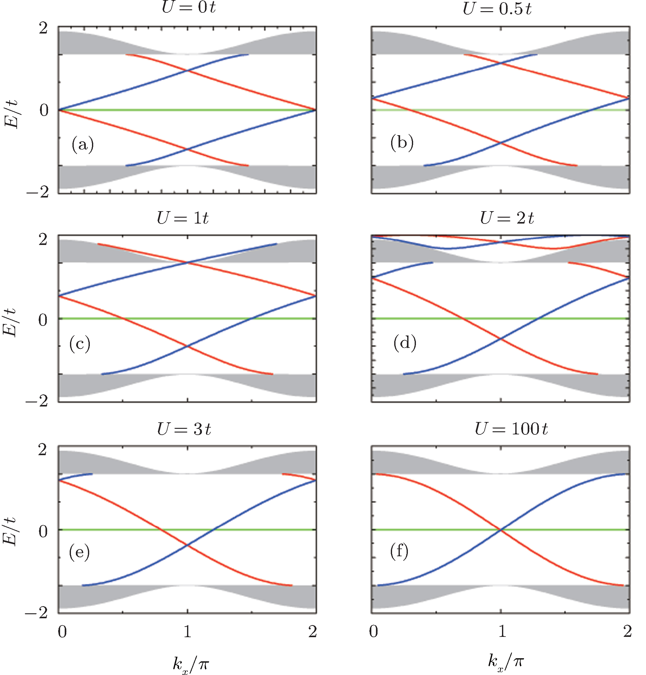
Fig. 10. Band structure of the strip Lieb lattice with the bearded edges and λ = 0.5t. The on-site energy U is applied on the outermost C-type atoms and is tuned to different values from 0 to 100t. Here, for clarity, only the edge modes localized near the upper boundary are shown. The red (blue) lines correspond to the edge states for the spin-up (spin-down) part. The green line corresponds to the flat bands.

Fig. 11.

Figure Option ViewDownloadNew Window

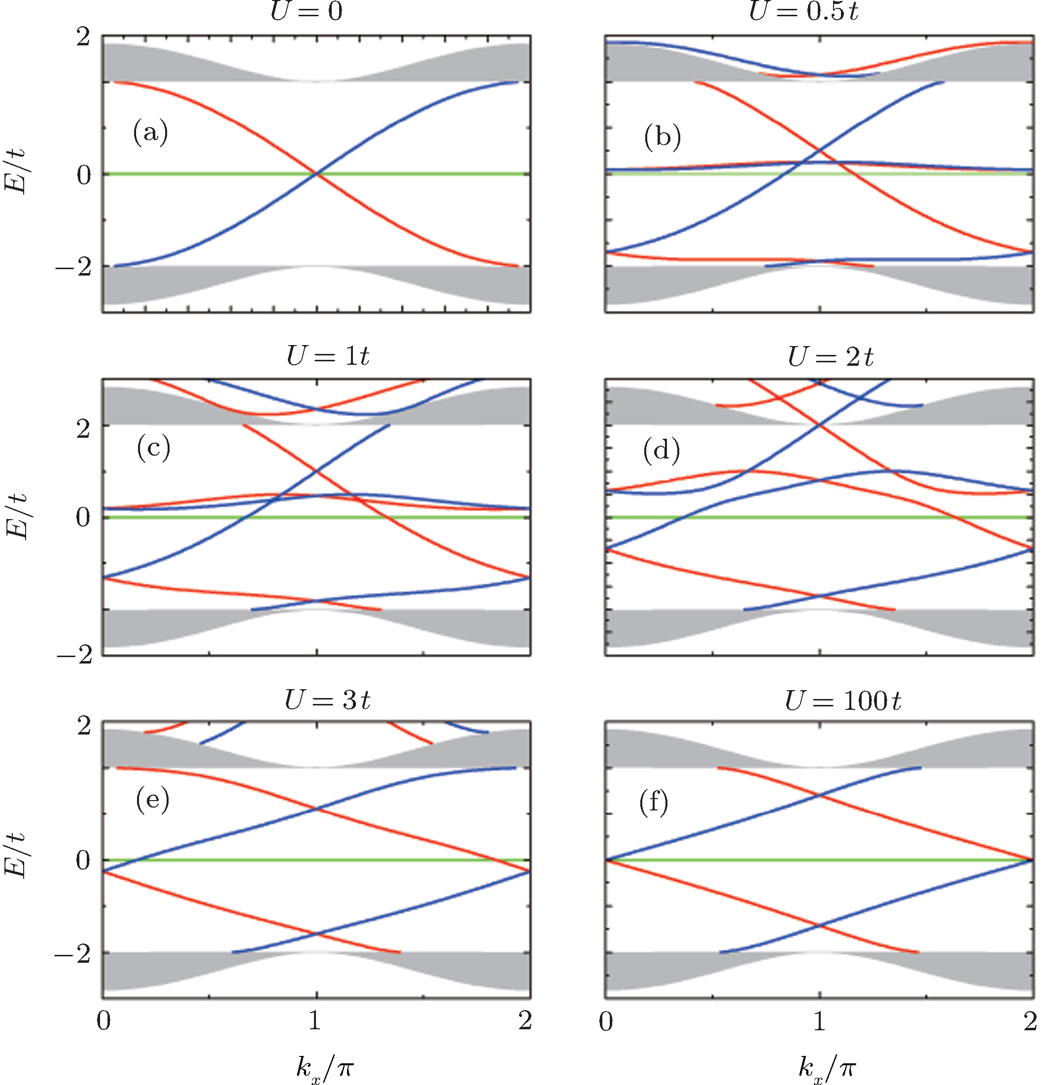
Fig. 11. Band structure of the strip Lieb lattice with the straight edges and λ = 0.5t. The on-site energy U is applied on the outermost A- and B-type atoms and is tuned to different values from 0 to 100t. Here, for clarity, only the edge modes localized near the upper boundary are shown. The red (blue) lines correspond to the edge states for the spin-up (spin-down) part. The green line corresponds to the flat bands.

In this paper, we re-examine the edge modes of the QSH effect on the Lieb lattice under different boundary geometries. For a two-dimensional Lieb lattice, when ISO coupling is introduced, two topologically nontrivial bulk gaps are opened between the bulk conduction and flat bands and between the bulk valance and flat bands, respectively. It will give rise to the QSH effect characterized by two pairs of gapless helical edge states within the bulk gap. We derive analytically the spectrum and wave function of edge modes based on the tight-binding model.

Firstly we discuss the edge modes on the Lieb lattice with a semi-infinite geometry. The straight edge and bearded edge are considered, respectively. It is found that for the Lieb lattice with a straight edge, the edge mode is composed only from orbitals of the types A and B, while for the case with a bearded edge the type-C atom also contribute to the edge states of the QSH effect. For the case with λ = 0.5t, the edge states are completely localized on the outermost atoms for both the straight edge and the bearded edge. It is also found that for both the straight edge and the bearded edge, the localization lengths of the edge modes vary non-monotonically with the amplitude of ISO coupling λ.

Next, we focus on the finite size effect of helical edge states on the strip Lieb lattice with ISO coupling under three different kinds of boundary conditions, i.e., the straight, bearded and asymmetry edges. For a strip Lieb lattice with two straight edges, the ISO coupling induces the Dirac-like bulk states to localize at the edges to become the helical edge states with the same Dirac-like spectrum. It is indicated that in this case with the straight edges the Dirac-like edge modes evolve from the Dirac-like bulk states without ISO coupling. Most significantly, the analytical results show that in this case with two straight edges the gapless Dirac-like spectrum remains unchanged with decreasing the width of the strip Lieb lattice, and no gap is opened in the edge band. Thus, it is concluded that the finite size effect of QSH states is absent on the Lieb lattice in the strip geometry with the straight edges, while the width of the strip model is comparable to the localization length of the edge modes. This result is strikingly different from the finite size effect on the HgTe quantum well discussed previously.^[31]

For the strip Lieb lattice with bearded edges, a bulk gap is opened between the flat band and the conduction band (or the valence band top) when ISO coupling is neglected. The inclusion of ISO coupling makes the degeneracy of the flat bands for the spin-up (or spin-down) part decreases by 2. It is indicated that two sides edge modes for spin-up (or spin-down) on the strip Lieb lattice with the bearded boundaries may evolve from two flat bands without ISO coupling. In contrast to the case with the straight edges, the energy gap ΔE induced by the finite size effect is opened (at k_x = π) with decreasing the width of the strip with the bearded edges, and the finite size gap ΔE decays exponentially with the sample width and non-monotonically varies with λ. Likewise, for the strip Lieb lattice with asymmetry edges, the finite size effect of QSH states still occurs. However, the finite energy gap of the edge bands generically opens at other finite k_x rather than at k_x = π. Compared with the case under the bearded edges, the finite size gap in the strip lattice with asymmetry edges has a faster decay rate with increasing sample width for the same amplitude of ISO coupling λ.

Finally, we demonstrate the edge bands dispersion of the Lieb lattice can be controlled by applying an on-site potential U to the outermost atoms.