Nickel oxide (NiO) has been widely studied as a prototypical system undergoing metal–insulator transition^[1] and titanium dioxide (TiO₂) has been widely studied as a wide bandgap semiconductor.^[2] Recently, these oxides have been actively studied as a resistive random access memories (ReRAM) sandwich layer. ReRAMs have emerged as a strong contender to replace FLASH-based memories as the need to construct integrated circuits goes beyond the complementary metal-oxide-semiconductor transistor (CMOS) architecture. In studies concerning these systems, the transition metal oxide is treated as an ion conducting layer and is sandwiched between two inert metal electrodes. The mechanism behind its operation is named resistive switching. It is achieved by the formation and destruction of a conductive filament in the dielectric between two electrodes.^[3] The device works by first having the insulating switching material in a high resistance state. By applying the electroforming voltage, a conductive filament is formed which creates a low resistance state. When a lower voltage is applied, the conductive filament is destroyed and the device is returned to a high resistance state.^[4] From a viewpoint of first principles, there have been recent studies concluding specific properties of these devices. Sarhan et al.^[5] concluded that the oxygen vacancies filament in a Pt/NiO/Pt system is the main contributor to electronic transport. Oka et al.^[6] have found that for a NiO supercell with Ni and O defects, the carrier concentration of holes is controlled by the presence of oxygen defects around nickel defects. Yoo et al.^[7] calculated the ground state energies for a TiO₂ supercell with oxygen vacancies by using the hybrid functional and concluded that external strain can affect the formation of the conductive filament. Park et al.^[8] in their study of a TiO₂ supercell found that due to electronic charge redistribution, electron hopping might occur when oxygen vacancies interact with each other. The central tools used to visualize the conductive filament in all these studies start with the Kohn–Sham electron wave function obtained from a first principles density functional theory calculation, followed by the electron localization function which measures the likelihood to find an electron near a reference electron at a given point with the same spin.^[9] This would then be used to perform the Bader charge density analysis which is an algorithm to integrate the electronic charge density around ions.^[10] This method however neglects strongly correlated effects, which are relevant to the study of charge transfer. This is because the construction of the charge density from a ground state calculation with a Hubbard term, U as has been the case in the above-mentioned studies will not adequately take into account electron correlation commonly studied as self-energy effects. Its importance has been highlighted by Peng et al.^[11] who have determined that the strongly correlated effects in a NiO supercell affect transport properties during resistive switching. Other highlights regarding correlation effects include the construction of other beyond CMOS devices, for example the application of VO₂ to constructing a metal insulator transition tunnel junction.^[12,13]

Studying the momentum density, which is defined as the probability to observe electrons with momentum p, instead of just the charge density of these oxides, should provide a more accurate description of the charge transfer. The use of intense synchrotron radiation is able to image a momentum density as a few percent of the Fermi momentum.^[14] Since it samples the bulk properties of the sample, it allows one to observe the electron wavefunction in k-space, making it a very useful tool for studying the Fermi surface, particularly studying quasiparticles.^[15] This allows the study of correlation effects between electron density and momentum transfer in materials. It is also possible to study individual spin states in which the Pauli exclusion principle can be observed. Experimentally, the momentum density can be obtained by performing an x-ray Compton scattering experiment in which it is re-obtained from the observed differential scattering cross section. It is useful in testing the accuracies in band-structure models. The Compton profile is considered as a projection of the electron momentum density. If the energy and momentum transfers of the probe energies are larger than the binding energies of the sample, we can obtain quasiparticle peaks, satellite structure, discontinuity and renormalization factor from the momentum density, which can be used to obtain an insight into the electron-electron correlation around the Fermi surface break. For shallow d-orbital systems such as transition metals, the observations of these terms indicate a breakaway from an equilibrium ground state theory. This can be seen in momentum density calculations where it is observed that there is some agreement in the high momentum region but disagreement in the low momentum region.^[16] This problem has been improved with the Lam–Platzmann correction.^[17] Nevertheless, the agreement of theory with experiment by using this correction shows small improvements. Furthermore, there seem to be observed the fine structures in theoretical Compton profiles compared with the experimental results in Ref. [18]. The alkali and alkali-earth metals in particular have been actively studied for their correlation effects as they are closest to the homogeneous electron gas and have isotropic momentum distributions. Later on, Schulke et al.^[19] remarked that final state interaction effects must be taken into account according to the work performed on Li. The use of the GW (G is Green’s function and W is the screened Coulomb interaction) approximation (GWA)^[20] is said to improve the comparison with observation for the Compton profile.^[21] Compton profiles for Li,^[22] Be,^[23] Na,^[24] Cr,^[25] Ni,^[26] and Cu^[27] have been obtained from the GWA.

Other interesting studies of Compton profile include molecular hydrogen,^[28] helium-like krypton,^[29] and ionized boron.^[30] Studies of Compton profiles of transition metal oxides from the GWA are scarce. However, studies of other properties derived from GWA prove important. Massida^[31] has shown in studies of NiO and MnO partial density of states that the GWA shifts Ni energies towards O more significantly compared to Mn. Yamasaki^[32] has shown that for TiO and VO, the hybridization between 3d and 2p increases as a result of band narrowing by GWA while the energy gap becomes smaller in GWA studies of MgO and CaO. Jiang^[33] has shown in studies of GWA + U for NiO and MnO that the quasiparticle renormalization factor increases as the Hubbard term increases. Rödl^[34] shows that in studies of the late TMOs that the application of the GWA and the HSE functional creates insulating states instead of metallic via GGA. Sai G and Bang-Gui Li^[35] used the Tran–Blaha modified Becke–Johnson exchange potential to calculate the electronic structure and optical properties of rutile and anatase TiO2 and observed that the energy gaps are in better agreement with the experimental result via comparing this functional with GW calculations. Peng et al.^[36] studied the electronic structure of CdHg(SCN)4 by using the GWA and observed that the Cd 4d and Hg 5d orbitals contribute to the valence band bottom while the valence band top and conduction band bottom originate from C 2p, N 2p and S 3p orbitals. Rong et al.^[37] observed that a more accurate band gap of 3.5-4.0 eV can be obtained for hydrogenated silicene by using the GWA with the Heyd–Scuseria–Ernzerhof functional. Yi^[38] observed that the d-band energies at high symmetry points for Cu can be closer to experimental values via GWA. Lu et al.^[39] studied the band structure of BaS via GWA and observed that the 4d Ba states are valence states and BaS is a direct gap semiconductor. Liu^[40] calculated an effective interaction potential in a Hartee type potential via the correlation function produced by the Coulomb interaction of the electron in the equation of the one-electron Green’s function. This term can be used to characterize the correlation strength of the system. The authors in Ref. [41] studied the quantum confinement effects on the self-energy electrons and holes via the dynamical plasmon-pole approximation theory and observed that the Coulomb potentials increase as confinement size decreases.

Besides the study of Compton profiles, the one electron Green’s function method can be used to determine the ionization potential since the poles of the one-particle Green’s function correspond to the electron addition and removal energy and the smallest removal energy is just the ionization potential.^[42] Other methods to study the effects of self-energy in the ionization potential involve the Breit interaction and quantum electrodynamics (QED) terms.^[43,44] In these studies, the authors studied the Lamb shift for groups 1 and 11 neutral atom valence electrons. The ionization potential contains two terms, i.e., the vacuum polarization term obtained from the Uehling potential,^[45] which is strongly localized to the nuclear neighborhood and the self-energy term which can be treated by obtaining a complete set of one-particle states at the Dirac level then doing the Feynman diagram. An effective atomic potential in the Dirac problem was then used to simulate the Dirac-Fock valence eigenvalues in terms of QED.

In this work we report on the momentum distributions of NiO and TiO₂ obtained from the spectral function by using the GWA. We compare this excited state momentum density with its ground state density and conclude that the excited state momentum density will reduce the density in the low momentum region and increase it in the high region by ∼12% and ∼5% respectively for NiO and ∼10% in both regions for TiO₂. In the Fermi break, we have observed that the stark differences between the ground state and excited state are greater than 20% for NiO and 50% for TiO₂ respectively, which is due to the broadening of the spectral function in this region. We characterize the effect of momentum density from electron correlation effects with the quasiparticle renormalization factor. We perform crystalline calculations instead of supercells due to the restrictions of the GWA method, particularly the contour deformation technique^[46] in ABINIT,^[47,48] which is the software used in this work. To the best of our knowledge, this is the first time this calculation has been performed and will act as a basis for future works with supercells and vacancies.

From a Compton scattering experiment, the double differential scattering cross section is given by

We perform two studies on the Compton profiles of crystalline NiO and TiO₂. For NiO, we initialize a rock-salt structure with the lattice parameter given by 4.1684 Å. In order to increase the sample size, we perform integrations over 5 Monkhorst–Pack grids. The grids we chose are 9 × 9 × 9, −18 × 6 × − 18, −13 × 13 × − 13, −14 × 14 × − 14, and −15 × 15 × − 15. We find that the ground state energies and excited state energies for each of these grids at the Γ point are consistent with three and two decimal places respectively if initalized with the following parameters. For the ground state calculation we initialize the plane wave kinetic energy cutoff as 1700 eV with a tolerance at 10⁻¹² eV over 30 bands. The plane wave kinetic energy cutoff controls the number of plane waves at a given k-point while the tolerance will cause the self-consistent cycle to stop when the absolute difference between the total energy is doubled successfully. We use the cold smearing technique to take into account the occupation of the electrons in the d-orbitals.^[50] The k-point grids as mentioned above converged after 27, 23, 25, 25, and 22 self-consistent iterations respectively. For the excited state calculations, we use the contour deformation technique to obtain the spectral function. To construct the dielectric matrix, we initialize 30 imaginary and real frequency points between energies of 10 eV to −10 eV. Its plane wave kinetic energy cutoff is set to be 1700 eV with a tolerance of 10⁻¹² eV and a polarizability cutoff at 270 eV over 30 bands with 20 unoccupied bands. In the excited state case, the plane wave kinetic energy cutoff determines the cut-off energy of the plane-wave set used to represent the wave functions in the formula that generates the independent-particle susceptibility while the polarizability cutoff determines the cut-off energy of the plane-wave set used to represent the independent-particle susceptibility. Obtaining the dielectric matrix, we can then obtain the self-energy term in which we have set the plane wave kinetic energy cutoff to be 1700 eV and the spectral function consists of 1600 data points in the range from −13 to 13 eV. To check the convergence of the excited state calculations, we perform the routines recommended by ABINIT whereby an initial screening calculation will be used to determine the converged plane wave kinetic energy cutoff for the self-energy term. With this converged term, we would then proceed to determine the converged number of bands with the self-energy term. With these two terms, we can then proceed to determine the converged plane wave kinetic energy cutoff, the number of bands and polarizability cutoff sequentially, for the dielectric matrices, which would then be checked for convergence for the self-energy. Even though the size of the Monkhorst–Pack grid is in the range of 80 to 120 k-points, ABINIT only allows k-points taken from this grid to undergo contour deformation calculations. We thus choose three directions to construct the momentum distributions, specifically [101] with 30 k-points, [001] with 21 k-points, and [101] with 36 k-points. For TiO₂, we initialize a rutile structure with lattice parameters 4.5889 Å–4.4559 Å–2.9576 Å. As the rutile structure requires more atoms than the rock-salt structure, we choose 4 Monkhorst–Pack grids with the sizes of 8 × 8 × 8, 9 × 9 × 9, 10 × 10 × 10, and 11 × 11 × 11, respectively. For the ground state calculation, the plane wave kinetic energy cutoff is 176 eV with a tolerance of 10⁻⁹ eV over 30 bands. Convergence is achieved after 10 iterations. For both NiO and TiO₂, we use the Troullier–Martins pseudopotential with a highest angular momentum of 2 in this calculation. For the excited state calculation we constructe the dielectric matrix out of 30 imaginary and real frequencies in the range from −10 eV to 10 eV. We finally construct the self-energy calculation with a plane wave kinetic energy cutoff of 176 eV with a polarizability cutoff of 176 eV. The spectral function is constructed from 100 frequency points in the range from 5.44 eV to 32.65 eV. We sample 16 k-points along the directions [100] and [111] respectively. The calculations are conducted as a spin polarized antiferromagnetic system and it is found that there is no significant difference between spin up or spin down spectral functions.

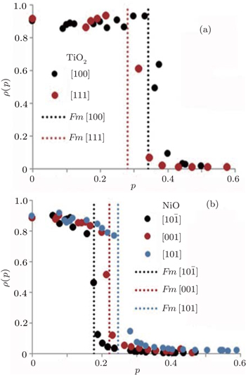
We firstly obtain the excited state Fermi energies, which are equivalent to the GWA valence band maxima from ABINIT to be 4.7565 eV for NiO and 14.1495 eV for TiO₂, respectively. The Fermi momentum or Fermi break is used to identify the break between occupied and unoccupied momentum densities^[21] as shown in Fig. 1 and has the unit of a.u. (The unit a.u. is short for atomic unit.)

Fig. 1.

	Figure Option ViewDownloadNew Window
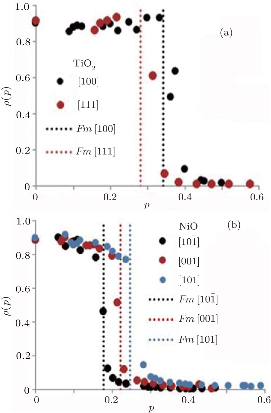	Fig. 1. GWA momentum densities (in units of e/a.u.) along the given directions and the locations of the Fermi break (vertical lines) as given in Table 1. NiO (b) momentum density shows significantly more broadening than TiO2 (a) above and below the Fermi break on the x axis (in units of a.u.).

We obtain the Fermi momentum by identifying the effective mass through fitting the valence band under the Fermi energy to a second order curve for all the directions of interest. For this analysis, we are only interested in the excited state bands as they will be used in our further analysis. The second order derivative of the inverse energy is given by

Table 1.

Table 1.

Table 1. Fermi momenta obtained along the given directions for NiO and TiO2. . NiO, pf/a.u. TiO2, pf/a.u. [001] 0.24 [100] 0.34 [101] 0.19 [111] 0.28 [101] 0.18

Table 1. Fermi momenta obtained along the given directions for NiO and TiO2. .

We obtain these densities by taking the value of the cumulant of the spectral function over all directions from a set of k-points at the Fermi energy.^[21] In the case of NiO, the spectral functions refer to the TM 3d band directly under the Fermi energy. The spectral functions above these energies refer to the unoccupied e_g band and under these energies refer to the O 2p bands, and have been reported to reproduce photoemission spectra. The contribution of the p-bands is small compared with the majority and minority d-bands for the top of the valence band. The GWA band gaps we have obtained are shown in Table 2 and are compared with previous GWA and experimental band gaps. Our result for NiO is more in agreement with model GW^[31,54] and LDA + U + GW^[33] calculations than with self-consistent GW^[51] calculations. Our TiO₂ band gap is also in the range of previously reported GW calculations and is in agreement particularly with DFT + GW.^[57]

Table 2.

Table 2.

Table 2. GWA band gaps for NiO and TiO2. . GWA band gap/eV Previous GWA band gaps/eV Experiment/eV NiO 3.27 3.75,[33] 4.8,[51] 5.5,[52] 3.7,[31] 2.4,[53] 3.6[54] 4.3,[59,60] 4.0[61] TiO2 3.15 3.59,[55] 3.78,[56] 3.13,[57] 3.40[58] 3.3,[62] 3.6[63]

Table 2. GWA band gaps for NiO and TiO2. .

At first glance, we observe that the Fermi–Dirac distribution is reproduced in NiO, which means that the impulse approximation is seemingly followed. TiO₂ almost follows this trend but has a constant momentum distribution at low momenta and falls in between the high and low momenta at the Fermi break. For NiO, there seem to be bigger curvatures before and after the discontinuity for each direction, respectively. This is followed by a region with zero occupancy until the Brillouin zone edge. In TiO₂ the curving is mainly seen after the Fermi break. This is almost similar to the Fermi liquid case where we would expect to see unity density at low momentum. The reason why we see bigger curvatures in NiO than in TiO₂ can be seen in the spectral functions as shown in Fig. 2 of the direction [101] for NiO and [100] for TiO₂ (these directions are representative of the other directions). For TiO₂ we can see that the origin of the constant momentum distribution in lower momenta as seen in Fig. 1 is due to a pile up of spectra at ∼13.4 eV before the Fermi energy. In the case of NiO, as the k-points increase, the spectral function of k-points approaching to the Fermi break and beyond tends to be more broadened. This is said to be due to the correlation terms shifting the occupancy from below to above the Fermi break. This confirms the role that correlation plays in broadening the spectral function and the discontinuity in the momentum distribution. The spectral function moves away from a Dirac-delta function which describes the behavior of the free noninteracting electron gas. This shows that the impulse approximation is not obeyed more strongly in this region than in other regions. This is consistent with experimental spectra where both a broadened quasiparticle peak and satellite structures are observed and explained as being a transition from a d₈ ground state to a d₇ final state via Anderson impurity calculations.^[52] Nevertheless, the spectrum agrees with the approximation in that it has a full quasiparticle weight with no satellite structures. This is typical of GWA calculations. Weak satellite structures have been observed in previous GWA calculations but by using muffin tin orbitals instead of plane waves. These structures manifest from peaks in the imaginary dielectric screening.^[49] The d₈–d₇ transition may be visible with application of ladder diagrams in the solution of GWA.^[52]

Fig. 2.

	Figure Option ViewDownloadNew Window
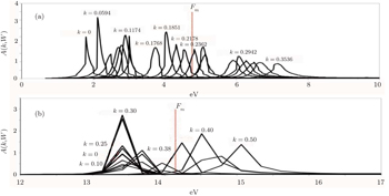
	Fig. 2. The spectral functions of k-points (in units of states/eV) along the directions of [101] for NiO (a) and [100] for TiO2 (b). The Fermi momentum is situated along overlapping spectral functions which explains the curving below and above the Fermi break in NiO. A pile up of spectra in lower momenta explains the constant momentum distribution as seen in Fig. 1.

We can thus explain the final state electron as a free noninteracting particle. This constructs the quasiparticle peak. This difference from spectra in lower momenta is caused by the interplay of the values of the frequency, ground state energy, real and self-energy as given in Eq. (11). It is well known that the energies under the Fermi energy in NiO are represented by the hybridization of p- and d-orbitals which are central to the discussion of strong correlation. A self-energy correction affects the reducing of hybridization with unoccupied 3d states.^[52] When the cumulant of these spectra is obtained to construct the momentum density, we find that the broadening contributes to its momentum density below the Fermi energy. This cumulant will naturally not be at unity at the Fermi energy owing to the curving of the momentum density. We perform a comparison of the momentum distribution of NiO in the GWA case with the occupation density obtained from its LDA calculation in Fig. 3.

Fig. 3.

	Figure Option ViewDownloadNew Window
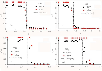
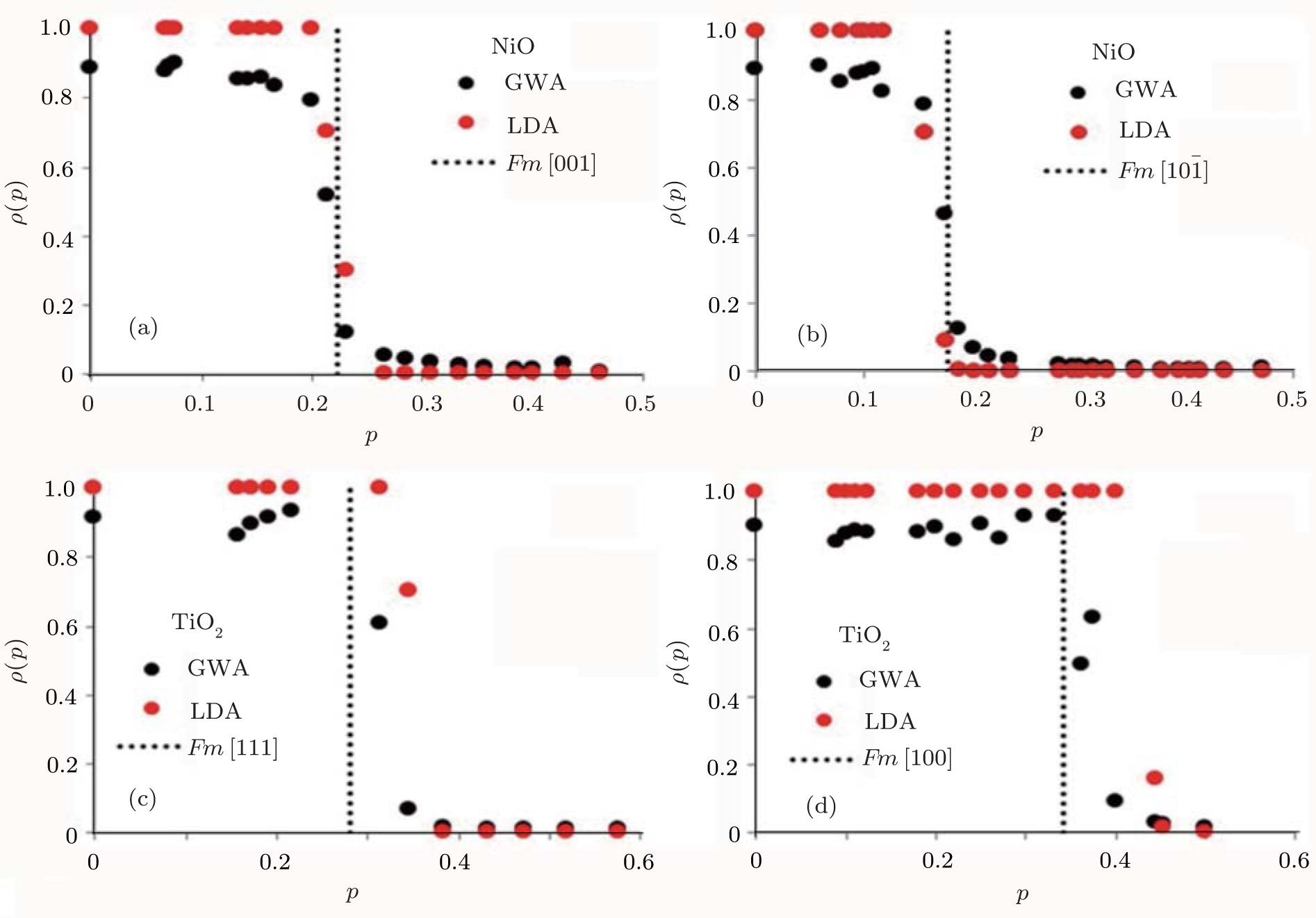	Fig. 3. A comparison between ground state (LDA) and excited state (GWA) momentum density (in units of e/a.u.) along [001] (panels (a) and (c)) and [101] (panels (b) and (d)) for NiO and [111] and [100] for TiO2. Low momentum densities show a large higher momentum. The most significant change is at the k-point below the Fermi momentum on the x axis (in units of a.u.).

In both directions, the self-energy makes the step function distribution in LDA resemble the Fermi–Dirac distribution. The GW momentum density shows that at the Fermi break, the k-points will be affected most. In both directions, from the origin to the k-point before the Fermi break, the GWA momentum density is ∼12% smaller than the LDA density. It differs by 35% and 20% respectively for the directions [001] and [101] respectively before the Fermi break and increases less than 5% above the Fermi break. For TiO₂we observe in both directions that GWA is ∼10% lower than LDA, GWA is ∼50% lower than LDA after the Fermi break and GWA is greater than LDA by ∼10% at high momenta. The decrease in low momenta from the ground state calculation is in line with what has been observed in experimental profiles, which is said to be a discrepancy with LDA calculations^[64] and has been observed in other work as well. Using the localized ion model, Chiba has calculated positron angular correlation curves of NiO single crystals and observed that the discrepancy with the experiment is fairly large in the low momentum region as well. This is observed in TiO₂ as well. Joshi calculated the Lam-Platzman correction based on free atom profiles and observed that the theoretical values are lower than experimental results in low momenta. They concluded that full atom profiles are inadequate to obtain the Compton profiles and stated a preference for Hartree–Fock (HF) methods to obtain difference profiles which are in better agreement with experimental results. This supports the use of GWA to obtain Compton profiles as it has been reported by Aryasetiawan and Gunnarsson.^[52] They stated that GWA can be regarded as HF without screening, in which the screening term leads to a larger reduction of gap due to long range correlations. They also reported the observation of a difference between the two cases compared with the substantial change in the wave function resulting from an increase of 1 eV in the LDA band gap to the GWA and a small downshift and bandwidth narrowing in d-bands and p-bands. In previous Anderson impurity calculations, spectra directly under the Fermi energy were interpreted as a 2p electron filling a 3d hole. Physically, this broadening is said to be due to the slowering of finite lifetime width of the spectral function reacting to change of momentum and energy transfer of probing energies. It involves final state electrons where the excited particle is polarized by the tightly bound core electrons and the electron hole it leaves behind. This polarization is directly obtainable from our first principles calculation (Eq. (9)) and used to obtain the final self-energy. Just from a simple comparison between ground state and excited state densities, it is obvious that polarization plays a significant role in the explaining of the momentum density. Thus, using the quasiparticle wave function as input to analyze the electron localization functions and Bader charge analysis would provide an insight into how the polarization would affect ion migration along the conducting filaments of ReRAMs.

With the momentum density, we can proceed to obtain the Compton profiles for both GWA and LDA cases. These profiles are compared with the experimental Compton profiles of Fukamachi et al.^[65] and Limandri et al.^[66] for NiO [001] and TiO₂ [111] with a Gaussian convolution of 0.55 a.u. and 0.15 a.u., respectively. The results are shown in Fig. 4. Our calculations for NiO are observed to follow the same trend as the experimental profile but it is seen to have a wide difference in the case of TiO₂ before the Fermi break. This difference can be explained by the above-mentioned constant momentum density in lower momenta for TiO₂ as a result of pile up of spectral function before the Fermi energy. This is not seen for NiO as there are bigger curvatures respectively before and after the discontinuity as a result of a broadened spectral function approaching to the Fermi break. Even though there is a large difference between the LDA and GWA momentum densities at the Fermi break for TiO₂, it is not reflected in the Compton profile as opposed to the NiO case. This is due to the small Gaussian convolution applied.

Fig. 4.

	Figure Option ViewDownloadNew Window
	Fig. 4. Compton profiles (in units of e/a.u.) obtained along the given directions for NiO (a) and TiO2 (b). For the NiO case, we see the existence of a more gradual drop to zero after the Fermi break. The Compton profile for TiO2 shows a slightly higher profile at the origin owing to a constant momentum density at lower momenta.

Finally we calculate the quasiparticle renormalization factor (QPRF), denoted by Z, as given in Table 3 at the k-points directly below the Fermi break. These values are obtained from Eq. (13). The gradient of the real energy is possible to be obtained since the real parts of the self-energy for both of the oxides at the Fermi energy and Fermi momentum have a linear relation. The quasiparticle renormalization factor for both NiO and TiO₂ are ∼0.6 and this is owed to the self-energy being of the same value as seen in Eq. (13). Nevertheless, a more in-depth look into the data reveals that the correlation part of the self-energy, denoted by Σ_c, is larger in magnitude for NiO than for TiO₂, while the exchange part of the self-energy, denoted by Σ_ex, is larger for TiO₂. This reveals that the correlation for NiO and exchange for TiO₂ each play a stronger role in the self-energy.

Table 3.

Table 3.

Table 3. Values of quasiparticle renormalization factor, Z obtained along the given directions for NiO and TiO2. For NiO, we have obtained these values for the 10th band and for TiO2 the 15th and 17th bands for [100] and [111], respectively. We have also included the exchange Σex and correlation Σc parts of the self-energy in our discussion of the quasiparticle renormalization factor. . NiO TiO2 [001] Z = 0.628 [100] Z = 0.662 (0.000,0.000,0.231) Σex = −10.748 eV (0.333,0.000,0.000) Σex = −19.896 eV Σc = −4.443 eV Σc = 2.903 eV [101] Z = 0.672 [111] Z = 0.697 (0.133,0.000,0.133) Σex = −10.995 eV (0.125,0.125,0.125) Σex = −15.052 eV Σc = −4.337 eV Σc = 1.724 eV [101] Z = 0.643 (0.125,0.000,−0.125) Σex = −11.029 eV Σc = −4.301 eV

Table 3. Values of quasiparticle renormalization factor, Z obtained along the given directions for NiO and TiO2. For NiO, we have obtained these values for the 10th band and for TiO2 the 15th and 17th bands for [100] and [111], respectively. We have also included the exchange Σex and correlation Σc parts of the self-energy in our discussion of the quasiparticle renormalization factor. .

In this work, we highlight the importance of the momentum density as a supplement to the established charge density analysis. NiO has long been known as a strongly correlated electron system compared with TiO₂ and this has been shown by comparing their momentum densities. For NiO, we observed that the curvatures before and after the Fermi break are due to the position of the break located along the overlapping spectral function. We relate this observation to the well known 3d–2p orbital hybridization of NiO and electron polarization as is calculated from the GWA. In comparison with ground state momentum densities, we observe a significant decrease and slight increase in the lower and higher momentum densities respectively. The most significant change is at the k-point below the Fermi break. We conclude that not only the momentum density supplement studies on systems using charge density analysis, but also the initialization of the quasiparticle wavefunction in the charge density would provide an analysis which takes into account the polarization of the electron, typical of GWA calculations. We then compare our calculations with previous experimental results and find that NiO is observed to follow the same trend as the experimental profile but it is seen to have a wide difference in the case of TiO₂ before the Fermi break. This difference can be explained by the abovementioned constant momentum density in lower momenta for TiO₂ as a result of pile up of spectral function before the Fermi energy. The quasiparticle renormalization factor reveals that the self energy of NiO has a strong correlation component compared with TiO₂ which has a strong exchange component. The calculated Compton profiles can be used to compare with experimental profiles obtained from Compton scattering experiments.