Laser-induced breakdown spectroscopy applied to the characterization of rock by support vector machine combined with principal component analysis
Yang Hong-Xing1, Fu Hong-Bo1, 2, Wang Hua-Dong1, 2, Jia Jun-Wei1, 2, Sigrist Markus W3, Dong Feng-Zhong1, 2, †,
Anhui Provincial Key Laboratory of Photonic Devices and Materials, Anhui Institute of Optics and Fine Mechanics, Chinese Academy of Sciences, Hefei 230031, China
University of Science and Technology of China, Hefei 230026, China
ETH Zürich, Institute for Quantum Electronics, Otto-Stern-Weg 1, CH-8093 Zurich, Switzerland


† Corresponding author. E-mail: fzdong@aiofm.ac.cn

Project supported by the National Natural Science Foundation of China (Grant No. 11075184), the Knowledge Innovation Program of the Chinese Academy of Sciences (CAS) (Grant No. Y03RC21124), and the CAS President's International Fellowship Initiative Foundation (Grant No. 2015VMA007).

Abstract
Abstract

Laser-induced breakdown spectroscopy (LIBS) is a versatile tool for both qualitative and quantitative analysis. In this paper, LIBS combined with principal component analysis (PCA) and support vector machine (SVM) is applied to rock analysis. Fourteen emission lines including Fe, Mg, Ca, Al, Si, and Ti are selected as analysis lines. A good accuracy (91.38% for the real rock) is achieved by using SVM to analyze the spectroscopic peak area data which are processed by PCA. It can not only reduce the noise and dimensionality which contributes to improving the efficiency of the program, but also solve the problem of linear inseparability by combining PCA and SVM. By this method, the ability of LIBS to classify rock is validated.

PACS: 52.25.Kn;52.50.Jm
1. Introduction

The laser-induced breakdown spectroscopy is a straightforward atomic emission spectroscopic technique that can provide rapid, multi-element detection with simple sample preparation. The laser-induced breakdown spectroscopy was first applied to the detection of hazardous gases and vapors in air at Los Alamos in the 1980s. Many researchers focused on the theory of laser-induced plasma (LIP),[1,2] electron density,[3,4] and laser–matter interaction which could improve the performance of LIBS.[58] Owing to its versatile advantages,[9] LIBS has been widely used in many fields from laboratory to practical applications such as industrial control,[1013] environment protection,[1417] agriculture,[1820] medical science,[21,22] and archaeology.[2325] Besides, LIBS has a trend of miniaturization, multiuse,[26] and using femtosecond laser to induce the plasma with some special characters.[27] Recently, qualitative analysis with chemometrics and pattern recognition has been conducted by many LIBS investigators and satisfactory results have been obtained by their work. In 2007, Sirven et al.[28] did many studies on the feasibility of rock identification at the surface of mars by remote laser-induced breakdown spectroscopy. They employed three chemometric methods: principal component analysis (PCA), soft independent modeling of class analogy (SIMCA), and partial least squares-discriminant analysis (PLS-DA) and obtained a best classification accuracy of 97.6%. In 2009, Yueh et al.[29] studied LIBS applied to the classification of biological samples by using 31 spectral lines of peak intensity, and they also gained good results by three methods: PLS-DA, hierarchical cluster analysis (HCA), and artificial neural network (ANN). In 2012, Cisewski et al.[30] built a support vector machine (SVM) model to evaluate the composition of suspect powders, particularly with respect to a possible content of Bacillus anthracis and obtained promising results.[30] De Lucia and Gottfried analyzed the explosive residues on organic substrates using LIBS data.[31] In China, many researchers, e.g., Yu et al.,[32] Tian et al.,[33] Wang et al.,[34] and Chen et al.[35] have contributed to LIBS for qualitative analyses through various methods such as PCA, PLS-DA, self-organizing mapping (SOM), and SVM. But the SVM combined with PCA has not been found to be applied to the LIBS data. In fact, the PCA is employed as a way of pretreating data and extracting features by many methods such as PLS-DA and SIMCA. This paper aims to classify rocks by LIBS data analyzed by SVM combined with principal component analysis.

2. Theoretical analyses
2.1. LIBS theory

The LIBS process involves many complex but independent areas such as laser–matter interaction, laser ablation of material, optical and thermodynamic properties of hot and ionized gas, and plasma propagation in a background gas.[5] When the plasma is in local thermal equilibrium (LTE) and there is no self-absorption, the emission intensity is given by

where F is the experiment parameter, Aij the transition probability for the spectral line from the energy level i to the level j, h the Planck constant, νij the frequency of the light emitted from the energy level i to the level j, N the number of particles of all energy levels with respect to the content of the specific element, gi the degeneracy of energy level i, U(T) the distribution function of the particles representing the total states of the particles at all levels at plasma temperature T, Ei the excitation energy of level i, and kB the Boltzmann constant. Equation (1) implies that the emission intensity depends linearly on the element concentration. However, in practice it is difficult to keep the plasma in LTE and self-absorption happens frequently.[36] Hence, the assumptions for Eq. (1) are difficult to realize and the element content and the spectrum intensity are not linear. Two typical ways are adapted to solve the problem. One is to employ the multivariate calibration methods,[3740] and the other is to calculate the self-absorption and correct the line intensity.
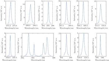
[41,42] But it can be assumed that there is some relationship between the intensity and the element concentration because the influence of self-absorption is constant for the same sample under identical experimental conditions. Instead, every selected line is a characteristic of the content of a specific element in the sample.
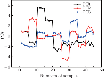
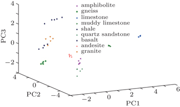
2.2. Principal component analysis (PCA)

PCA is often employed because it enables the decreasing of noise and dimensionality. The main ideal is that the raw data X can be decomposed into the product of two small matrices:

where the raw data X is an n × p matrix (n is the number of the samples, and p is the number of characteristics), T is the score matrix n × d (d is the number of principal components (PCs)), and L is the load matrix p × d. The diagonal elements of TTT are called eigenvalues λi. In this way, the raw data are mapped into new dimensions. The new data T is a linear combination of the original data X. The first PC can explain the highest variance of the raw data X because the PCA is based on maximal variance criterion. The second PC explains a little less variance than the first PC and the third again less than the second PC. Generally the first several PCs are sufficient when the sum of the PCs exceeds a threshold such as 90%, but it depends on the real situation. As a result, the dimension is reduced by abandoning the data which is dominated by noise.
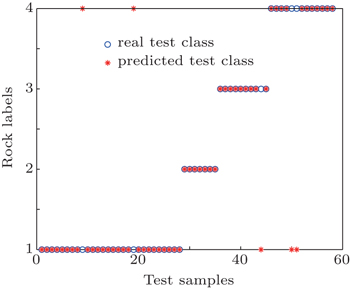
2.3. SVM

The SVM has many applications in statistics, in particular for classification. The main idea of SVM is to find the hyperplane that can best distinguish the data by maximizing the margin between the closest points in each class.[43] Considering that the raw data may be nonlinear, the kernel function of the radial basis function (RBF) is chosen as:

where σ2 is the RBF variable, which is set by experience initially and determined by cross validation in the end.

3. Experimental setup and data pretreatment
3.1. LIBS experimental system

The classic experimental setup is adopted to acquire the spectral data as shown in Fig. 1.

Fig. 1. Schematic experiment setup.

The Nd:YAG laser (Quantel model ULTRA50) is operated at the fundamental wavelength of 1064 nm. The laser pulse energy is fixed at 50 mJ, pulse width is 7ns, and the repetition frequency is 0.5 Hz. The laser is reflected by a 45° mirror first, and focused on the sample surface by an optical lens (lens 1) with 100-mm focal length. When the laser power density exceeds the ablation threshold of the material (typical 107 W/cm2), a plasma is formed, emitting dazzling light which contains continuous background light and characteristic spectral lines from energy level transitions. The focused spot diameter is (0.75018±0.06931) mm measured by Abbe comparator (Shanghai model 6W810115) for 5 different spots. Thus the laser power density can be calculated to be 1.26 × 10⁹ W/cm2. The emitting light is collected by a spectrometer (Avantes model AVS-DESKTOP-USB2) through an optical lens (lens 2) and a fiber. The spectrometer range is between 180 nm and 610 nm with a spectral resolution of about 0.05 nm. From the experiences of our group, the spectral integral time of the experiment is set to be 1.03 ms, and the delay time between the laser pulse and the collection of the emission is set to be 1.05 μs.

The experiment is performed with nine types of rock debris (Amphibolite, Gneiss, Limestone, Muddy Limestone, Shale, Quartz Sandstone, Basalt, Andesite and Granite). Figure 2 shows the approximate size of the rock debris sample which is pressed into a tablet under a pressure of 20 MPa for 5 min. Fourteen characteristic lines are picked corresponding to the emissions by Mg, Ca, Fe, Al, Si, and Ti, as listed in detail in Table 1. After that, the peak areas of the fourteen lines can be calculated. Because the intensity of Na emission line is higher than others and the spectrograph can become saturated easily, the Na lines are not included. From Fig. 3, it can be seen that all 14 emission lines do not have obvious self-absorption. But as is well known, the 14 emission lines are still influenced more or less by self-absorption, but it is hopeful to be partly overcome by the program since it is assumed that the degree of self-absorption of the same sample is the same. The 45 rock debris samples are chosen in the experiment. The first 5 laser pulses are employed to clean the sample surface and the subsequent 20 pulses are used to obtain an average spectrum.

Fig. 2. Photograph of a rock debris sample.
Table 1.

Selected emission lines for analysis of LIBS spectrum of rock debris.

.
Fig. 3. Outlines of the 14 selected analytical lines.
3.2. Data pretreatment

The data selected from the total emission spectrum are the peak areas which are calculated from the spectra directly rather than the peak intensities of the 14 spectral lines. So the spectrometer does not need high spectral resolution. As an example, the intensity of the Ca line at 585.74 nm corresponds to 4956.60 a.u. (a.u. is short for arbitrary unit) as shown by the measurement in Fig. 4, while the Lorentz fitting yields 6280.05 a.u.

After the spectral peak areas are calculated, the data are normalized to reduce fluctuations caused by laser energy, irregularity of the sample surface and interference from outside. For each sample, the normalization is

where Di is the peak area data calculated from the spectrum and Xi is the data after normalization. To build a better SVM training model, it is necessary to exclude singular samples. Lastly, the SVM yields the final classification after application by PCA.

Fig. 4. Lorentz Fitting of Ca emission line at 585.74 nm.
4. Results and discussion
4.1. Result of PCA

PCA yields valuable information about the rock debris. At first it is necessary to determine the number of PCs. The first three PCs have explained over 90% of the variance of the original data and the fourth PC explained only 4.83% (see Table 2 for the details), so only the first three PCs are chosen. As a result, the dimensionality is reduced from 14 to 3.

Table 2.

Rates of raw data variance explained by PCs.

.

As figure 5 implies, we can obtain a rough estimate about the classification ability on the basis of the first three PCs. Since each kind of rock debris has 5 samples, a visible saltation appears every 5 numbers at the boundaries of different kinds of rock debris. The PCs vary widely for different types of rock debris and change little within the same type. The first four kinds of rock debris can be easily distinguished by PC1. The sixth, eighth and ninth kinds can be set apart by PC2. The rest can be marked differently by PC3. The only minor defect is the fifth and ninth kind that may be mixed up. But the fifth and ninth kinds may be distinguished by PC4. However, it is possible that PC4 fails to get them apart for the following reasons: Firstly, it can be seen that the third PC has become smooth while it can explain 14.75% of the original variance and the fourth PC only 4.83%. Secondly, PCs are the linear combination of the original data. If the original data are nonlinear, the PCA is bound to fail no matter how many PCs are used.

Fig. 5. Variations of the first three PCs with the number of samples. Each kind of rock is represented by 5 samples.

Figure 6 shows the scatters of the first three PCs of nine kinds of rock debris. The figure demonstrates that the nine kinds of rock debris are well distinguished and all five samples of each debris are gathered in a very small area. Only shale and granite (the fifth ◼ and the ninth ▲) show a pair of overlapped points. Possible reasons of the overlapped points of shale and granite are below.

Fig. 6. Scatter of first three PCs of nine kinds of rock debris.
Table 3.

Element content (by weight percent) of typical granite and shale.

.
4.2. Results of SVM combined PCA

To overcome the defect of PCA, the SVM is employed to classify the nine rock debris based on the result of PCA. In addition, the RBF kernel function is chosen because of its ability to deal with nonlinear data. Five samples selected from each kind of rock debris are divided into three training samples and two test samples randomly. The first three PCs are chosen as the input data of SVM. To obtain a steady and reliable model, k-fold cross validation is operated to optimize the model. Two factors C and σ2 vary from −1024 to +1024 in steps of 0.01 and from −100 to +100 in steps of 0.01 respectively. By this progress, the best optimized penalty coefficient C = 1024 and the RBF variable σ2 = 2.46 are gained. The classification result is shown in Fig. 7.

It can be seen from Fig. 7 that all 18 test samples have been classified correctly with an accuracy of 100%, and also granite and shale are successfully classified. This good result can be explained by the following reasons.

Fig. 7. Classification results of SVM combined with PCA for nine kinds of rock debris.

The whole program takes a few minutes (430.36 s), in which cross validation occupies much time (429.68 s, 99.84% of the total time). However, we should also realize that the model built by the training samples has been over trained. This can be derived from the penalty coefficient C of 1024 which is the highest among the numbers set by the program. The main reason is that the 14 selected emission lines cannot represent the biggest difference of the different kinds of rocks. The same situation happens during the identification of plastics.[32] The SVM is a supervised learning, so the training model is the key which determines the program performance. If the training samples exhibit much noise, SVM must take a large penalty coefficient to classify them. Hence the noise reduction of the input data achieved by PCA keeps the training model more practical. The selection of the analytical emission lines plays a fundamental role in the training.

Fig. 8. Classification results of SVM combined with PCA for four real rock samples.
5. Conclusions

LIBS is demonstrated to be feasible for the analysis of rock during geological exploration due to its versatile advantages. The peak area instead of peak intensity is a suitable way to acquire useful data from LIBS spectra. For rock debris, the classification accuracy is 100%, while for real rock the accuracy decreases to 91.38%. LIBS yields rich and valuable spectral information. By combining PCA and SVM, it can not only reduce the noise and dimensionality which is helpful to improve the efficiency of the program, but also solve the problem of linear inseparability. This method can be adapted to classify the samples which have multivariate characters with not much noise. The crucial question is how to select the most appropriate emission lines for the analysis which can represent for the biggest difference among the different kinds of rocks in order to build a more practical model. Here we employ 14 analysis lines selected by the prior knowledge of the elements contained in the rock material.

Reference
1Cao YLiu X LXian W DSun S HSun M ZDing P JShi Y CLiu Z YHu B T 2015 Chin. Phys. Lett. 32 035203
2Chen HLan HChen Z QLiu L NWu TZuo D LLu P XWang X B 2015 Acta Phys. Sin. 64 075202 (in Chinese)
3Zhang Z MZhang BWu F JHong WTeng JHe S KGu Y Q 2014 Acta Phys. Sin. 64 105201 (in Chinese)
4Zhang LDong Q LWang S JSheng Z MZhang J 2010 Chin. Phys. 19 078701
5Yu JMa Q LMotto-Ros VLei W QWang X CBai X S 2012 Front. Phys. 7 649
6Li Z CZheng JJiang X HWang Z BYang DZhang HLi S WWang FPeng X SYin Q 2011 Chin. Phys. Lett. 28 125202
7Li Z CZheng JDing Y KYin QJiang X HLi S WGuo LYang DWang Z BZhang H 2010 Chin. Phys. 19 125202
8Zhao YZhu TWei M XXiong GSong T MHu Z MHuang C WShang W LYang G HZhang J Y 2012 Chin. Phys. Lett. 29 085202
9Noll R2012Laser-Induced Breakdown Spectroscopy: Fundamentals and ApplicationsBerlinSpringer7
10Lorenzen C JCarlhoff CHahn UJogwich M 1992 J. Anal. Atom. Spectrom. 7 1029
11Palanco SLaserna J 2000 J. Anal. Atom. Spectrom. 15 1321
12Kurihara MIkeda KIzawa YDeguchi YTarui H 2003 Appl. Opt. 42 6159
13Noll RMönch IKlein OLamott A 2005 Spectrochim. Acta 60 1070
14Tran MSmith B WHahn D WWinefoner J D 2001 Appl. Spectrosc. 55 1455
15Hettinger BHohreiter VSwingle MHahn D W 2006 Appl. Spectrosc. 60 237
16Bossu MHao Z QBaudelet MYu JZhang ZZhang J 2007 Chin. Phys. Lett. 24 3466
17Zhu G ZGuo L BHao Z QLi C MShen M SLi K HLi X YLiu J GZeng X YLu Y F 2015 Acta Phys. Sin. 64 024212 (in Chinese)
18Sirven J BBousquet BCanioni LSarger LTellier SPotin-Gautier MLe Hecho I 2006 Anal. Bioanal. Chem. 385 256
19Bousquet BSirven J BCanioni L 2007 Spectrochim. Acta 62 1582
20Senesi GDell'Aglio MGaudiuso RDe Giacomo AZaccone CDe Pascale OMiano TCapitelli M 2009 Environmental Research 109 413
21Morel SLeone NAdam PAmouroux J 2003 Appl. Opt. 42 6184
22Corsi MCristoforetti GHidalgo MLegnaioli SPalleschi VSalvetti ATognoni EVallebona C 2003 Appl. Opt. 42 6133
23Burgio LMelessanaki KDoulgeridis MClark R J HAnglos D 2001 Spectrochim. Acta 56 905
24Giakoumaki AMelessanaki KAnglos D 2007 Anal. Bioanal. Chem. 387 749
25Kaszewska E ASylwestrzak MMarczak JSkrzeczanowski WIwanicka MSzmit-Naud EAnglos DTargowski P 2013 Appl. Spectrosc. 67 960
26Wang S HLi Z LSun C LLi Z WMen Z W 2014 Acta Phys. Sin. 63 205204 (in Chinese)
27Zhang NBao W XYang J HZhu X N 2013 Chin. Phys. 22 054209
28Sirven J BSalle BMauchien PLacour J LMaurice SManhes G 2007 J. Anal. Atom. Spectrom. 22 1471
29Yueh F YZheng H BSingh J PBurgess S 2009 Spectrochim. Acta 64 1059
30Cisewski JSnyder EHannig JOudejans L 2012 J. Chemometr. 26 143
31De Lucia F CGottfried J L 2012 Appl. Opt. 51 B83
32Yu YHao Z QLi C MGuo L BLi K HZeng Q DLi X YRen ZZeng X Y2013Acta Phys. Sin.62215201(in Chinese)
33Tian YWang Z NHou H MZhai X WCi X HZheng R E 2012 Spectrosc. Spect. Anal. 32 2027
34Wang Q QLiu KZhao H 2012 Chin. Phys. Lett. 29 044206
35Chen X LDong F ZTao G QLi Y JShe M JFu H BNi Z BWang J G 2013 Chin. J. Lasers 40 1215001
36Cristoforetti GDe Giacomo ADell'Aglio MLegnaioli STognoni EPalleschi VOmenetto N 2010 Spectrochim. Acta 65 86
37Sun L XYu H BXin YCong Z B 2010 Spectrosc. Spect. Anal. 30 3186
38Stipe C BHensley B DBoersema J LBuckley S G 2010 Appl. Spectrosc. 64 154
39Clegg S MSklute EDyar M DBarefield J EWiens R C 2009 Spectrochim. Acta 64 79
40Laville SSabsabi MDoucet F R 2007 Spectrochim. Acta 62 1557
41Bredice FBorges F OSobral HVillagran-Muniz MDi Rocco H OCristoforetti GLegnaioli SPalleschi VPardini LSalvetti ATognoni E 2006 Spectrochim. Acta 61 1294
42Bulajic DCorsi MCristoforetti GLegnaioli SPalleschi VSalvetti ATognoni E 2002 Spectrochim. Acta 57 339
43Cristianini NShawe-Taylor J2000An introduction to support vector machines and other kernel-based learning methodsCambridgeCambridge University Press93
44Liu Y FDing Y JPeng Z MHuang YDu Y J 2014 Acta Phys. Sin. 63 205205 (in Chinese)