
Effect of turbulent atmosphere on the on-axis average intensity of Pearcey–Gaussian beam
[Boufalah F, Dalil-Essakali L, Nebdi H, Belafhal A†,  ]
]
]
|
|


† Corresponding author. E-mail:
The propagation characteristics of the Pearcey–Gaussian (PG) beam in turbulent atmosphere are investigated in this paper. The Pearcey beam is a new kind of paraxial beam, based on the Pearcey function of catastrophe theory, which describes diffraction about a cusp caustic. By using the extended Huygens–Fresnel integral formula in the paraxial approximation and the Rytov theory, an analytical expression of axial intensity for the considered beam family is derived. Some numerical results for PG beam propagating in atmospheric turbulence are given by studying the influences of some factors, including incident beam parameters and turbulence strengths.
Diffraction catastrophe theory is the theoretical foundation for generating accelerated beams such as Airy beams which are derived from fold diffraction catastrophe,[1] Pearcey beams from cusp diffraction catastrophe,[2] regular polygon beams from Thom’s elliptic umbilics,[3,4] and other accelerated beams that were recently introduced.[5–7] Hence, based on the relation between diffraction integrals and catastrophe polynomials,[8,9] a general canonical catastrophe integral can be obtained.[6] So, to realize a diffraction catastrophe, one of the methods is to use phase-only diffraction patterns. The key task of such a method is to produce an appropriate phase mask. Hence, the corresponding phase profile masks can be obtained on the basis of caustic characteristic diffraction pattern. For example, as is well known, 3/2 phase only pattern can generate Airy beams,[10] observed experimentally for the first time by Siviloglou et al.,[11] and the quartic polynomial exponent phase can generate Pearcey beams.[12] These last new kinds of paraxial beams were formulated by Ren et al.,[13] based on the Pearcey function of catastrophe theory.
The propagating form of the Pearcey beam has several noteworthy properties, some of which are reminiscent of not only Airy beams, but also Gaussian and Bessel beams. Like the Bessel beam and Airy beam, a pure Pearcey beam has infinite energy, but can be made finite by modulating the Pearcey function with a Gaussian one in real space, which does not significantly change the beam properties. Earlier, it was shown that the Pearcey beams are auto-focusing and self-healing after being distorted by obstacles.[12] In a recent paper, a virtual source was proposed to generate the Pearcey beams.[14] In Ref. [15] Pearcey beams were generalized into half Pearcey beams and it is shown that such beams, which are form-invariant,[12,15,16] propagate with acceleration and auto-focusing.
Recently, a lot of attention was paid to studying the propagation of some laser beams in a turbulent atmosphere[17–28] because of their large applications in optical communications, imaging systems and remote sensing.[29–32] As is well known, when a laser beam propagates in the atmosphere, it produces random variations in amplitude and phase of the electric field caused by random changes of the refractive index. In our research group, the propagations of Li’s flat-topped beams,[33] Bessel-modulated Gaussian beams,[34] Superposition of Kummer beams,[35] truncated modified Bessel modulated Gaussian beams with quadrature radial dependence (MQBG),[36] and Li’s flattened Gaussian beams[37] in turbulent atmosphere were investigated. In Ref. [12], the propagation of PG beams in free space has been given. But to our knowledge, the propagation of PG beams in turbulent atmosphere has not been studied elsewhere.
In this paper, our interest is to study the propagation characteristics of PG beams through a turbulent atmosphere. The rest of this paper is organized as follows. In Section 2, an analytical expression of the average intensity of the considered beams is given based on the extended Huygens–Fresnel integral formula in the paraxial approximation and on the Rytov theory. An approximate analytical axial intensity distribution is derived in Section 3. We present some numerical simulations in Section 4. Finally, a conclusion is drawn from the present work in Section 5.
In this section, we give the expression of the one-dimensional average intensity of the PG beams after propagating in turbulent atmosphere. The Pearcey function is defined by an integral representation[38,39] as

The field distribution of the PG beams in the Cartesian coordinates (x1,y1, z) at the plane z = 0 is given by[12]
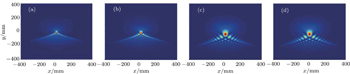
We illustrate in Figs.
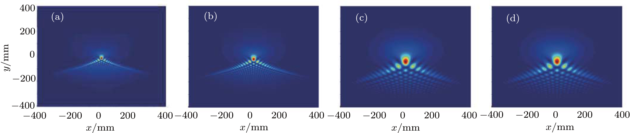 | Fig. 1. Incident transverse intensities of PG beams in source plane (z = 0) for ω0 = 0.5 mm and λ = 1550 nm with (a) x0 = y0 = 1 × 10⁻² mm, (b) x0 = y0 = 1.2 × 10⁻² mm, (c) x0 = y0 = 1.6 × 10⁻² mm, and (d) x0 = y0 = 3 × 10⁻² mm, respectively. |
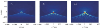
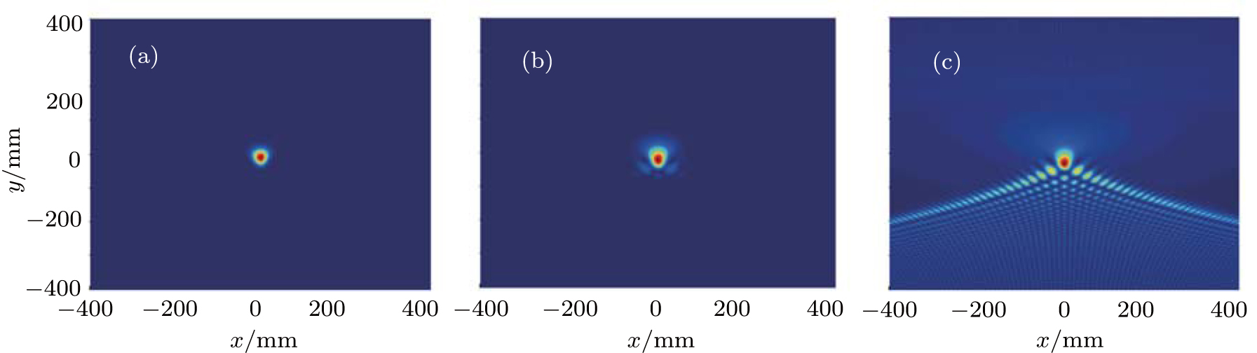
 | Fig. 2. Incident transverse intensities of PG beams in source plane (z = 0) for ω0 = 1 mm and λ = 1550 nm with (a) x0 = y0 = 1 × 10⁻² mm, (b) x0 = y0 = 2 × 10⁻² mm, and (c) x0 = y0 = 3 × 10⁻² mm, respectively. |
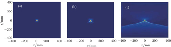
 | Fig. 3. Incident transverse intensities of PG beams in source plane (z = 0) for λ = 1550 nm, x0 = y0 = 1.064 × 10⁻² mm with (a) ω0 = 5 × 10⁻² mm, and (b) ω0 = 0.1 mm, and (c) ω0 = 3 mm, respectively. |
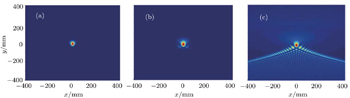
 | Fig. 4. Incident transverse intensities of PG beams in source plane (z = 0) for λ = 1550 nm, x0 = y0 = 2 × 10⁻² mm with (a) ω0 = 5 × 10⁻² mm, (b) ω0 = 0.1 mm, and (c) ω0 = 3 mm, respectively. |
Based on the extended Huygens–Fresnel integral formula in the paraxial approximation and on the Rytov theory, the expression of the electric field of the PG beams after propagating in a turbulent atmosphere is written as[40]

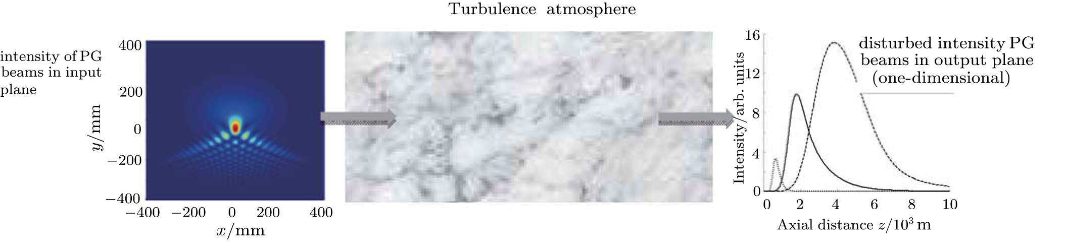 | Fig. 5. A schematic propagation of the PG beams in a turbulent atmosphere optical system. |
In the following, we only consider a one-dimensional expression of the electric field of the PG beams at the z = 0 plane, which is expressed as


In this section, we derive the axial intensity distribution of PG beams in turbulent atmosphere using Eq. (


Finally, after tedious calculations, the analytical expression of the axial intensity distribution of PG beams in turbulent atmosphere is written as
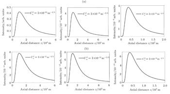
We illustrate in Fig. 
 | Fig. 6. Plots of on-axis average intensity versus the propagation distance z of PG beam for (a) x0 = 2 × 10⁻² mm and (b) x0 = 6 × 10⁻² mm, three values of the turbulent strengths, λ = 632.8 nm, and ω0 = 1 mm, respectively. |
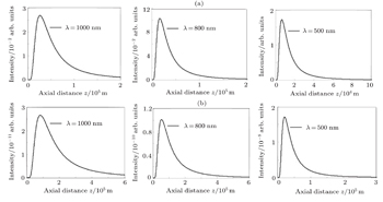
To show how the beam wavelength affects the on-axis average intensity, we illustrate the variations of on-axis average intensity with propagation distance z in Fig. 
 | Fig. 7. Plots of on-axis average intensity versus propagation distance z of PG beam for (a) ω0 = 1 mm and (b) ω0 = 0.5 mm, three values of λ,  |
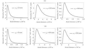
Figure
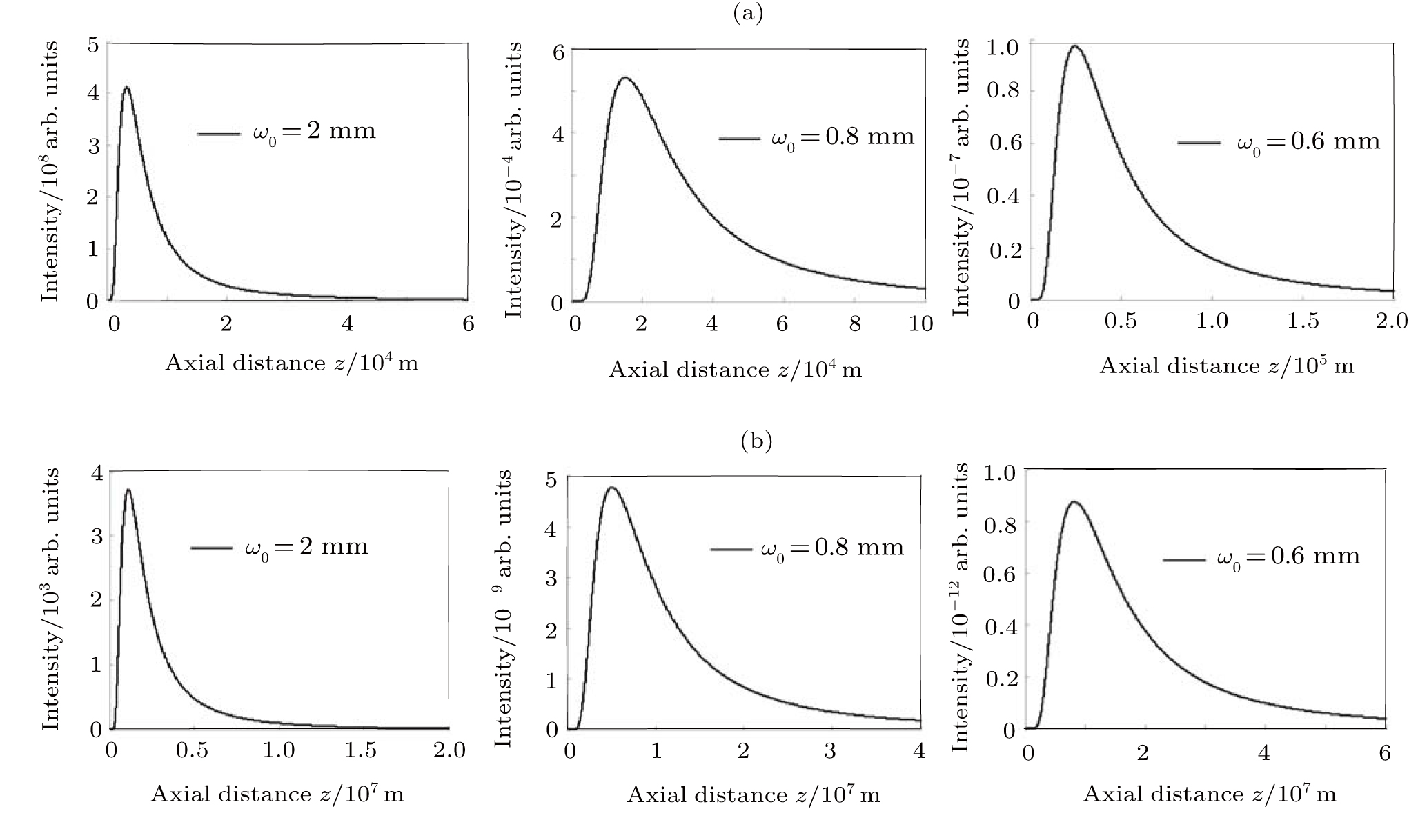 | Fig. 8. Plots of on-axis average intensity versus the propagation distance z of PG beams with three values of ω0, λ = 632.8 nm, x0 = 2 × 10⁻² mm for (a)   |
In this work, we derive an analytical expression of the axial intensity for PG beams, based on the extended Huygens–Fresnel integral formula in the paraxial approximation and on the Rytov theory, in turbulent atmosphere. Our numerical simulations shown that the PG beams with larger wavelength and smaller waist are less affected by the atmospheric turbulence, which is useful for applications in the field of optical communication for a long distance.
| 1 | |
| 2 | |
| 3 | |
| 4 | |
| 5 | |
| 6 | |
| 7 | |
| 8 | |
| 9 | |
| 10 | |
| 11 | |
| 12 | |
| 13 | |
| 14 | |
| 15 | |
| 16 | |
| 17 | |
| 18 | |
| 19 | |
| 20 | |
| 21 | |
| 22 | |
| 23 | |
| 24 | |
| 25 | |
| 26 | |
| 27 | |
| 28 | |
| 29 | |
| 30 | |
| 31 | |
| 32 | |
| 33 | |
| 34 | |
| 35 | |
| 36 | |
| 37 | |
| 38 | |
| 39 | |
| 40 | |
| 41 |