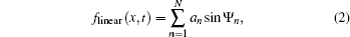
1. IntroductionThere are many types of ocean currents with different spatial and temporal scales on the ocean surface. They are essential components of the ocean circulation system and the relevant ecosystem. Ocean currents play important roles in the transportation of heat, mass, momentum, nutrients and energy.[1]
Remote sensing by satellite is the ideal technology for studying hydrodynamic dynamics of the ocean surface. It can obtain daily and weekly global coverage data with high revisit frequency and high spatial resolution by synthetic aperture radar (SAR). Chapron et al.,[2] and Johannessen et al.[3] derived an indirect retrieval algorithm for ocean surface current from the SAR Doppler frequency shift, as observed in the imagery. This method can only retrieve ocean current velocity in the range direction and the current direction is only derived with the aid of ancillary information. Marghany[4] improved the retrieval method for ocean current for RADARSAT-1 measurements by SAR imagery through using a method based on wavelength discrepancy and multiple looks at different frequencies. Some relevant studies and publications have reported ocean current retrieval results in different geographical areas by using TerraSAR-X, and Envisat ASAR.[5,6] Unfortunately, there is no method to directly measure ocean currents by sensors on satellites presently.
For ocean surface current, it is necessary to study the remote sensing mechanism, where the effect of the ocean current on electromagnetic (EM) backscattering of the sea surface is a key step to solve the problem. The surface current can modulate the EM backscattering signal because the current can change the wave parameters such as wave spectrum, wave height, wave period and other relevant variables. As a case study, the shoaling wave experiment (SHOWEX) shows that there is a drift of the wind wave spectrum with the mean wind direction because of horizontal current shear at the edge of the current front.[7] Therefore, there is an obvious correction of the amplitude dispersion relation, which is needed in the shallow water area.[8] Numerical results for the time evolution of the shallow water wave show that offshore currents can occur when a wave propagates and breaks in topographically changing shallow water, whereas the intensity and scale of the offshore current can be weakened by negative feedback because of the wave–current interaction.[9]
A fundamental objective of our study is to establish a high accuracy sea surface model. The fractal geometry method has characteristics of both periodicity and stochasticity. It can therefore be easily used to simulate the sea surface. Many recent studies focused on the fractal sea surface model and have used this approach to study EM scattering at the sea surface.[10–17] In this paper, the one-dimensional linear and nonlinear fractal sea surface models are used to derive wave–current coupled models, based on the wave–current interaction mechanism.
Nonlinear wave–current coupled models are derived in Section 2. An error analysis of our models is given in Section 3. Numerical simulation of the effect of the ocean current on the waves is given in Section 4. Conclusions are shown in Section 5.
2. One-dimensional wave–current coupled modelsStarting with linear and nonlinear fractal sea surface models, linear and nonlinear wave–current models are derived in this section.
2.1. Linear fractal sea surfaceFor a one-dimensional linear irrotational flow system, the velocity potential function is

where
ω is the radian frequency of the ocean wave. The linear wave derived from Eq. (
1) is given by
where
N is the number of wave components,
Ψn =
knx –
ωnt +
φn,
an,
kn,
ωn, and
φn are the amplitude, wave number, radian frequency, and phase of the
n-th wave components, respectively. A given wave propagates in the
x direction. Time is represented by
t in units of seconds. Wave numbers are given by

where
λn is wavelength of the
n-th wave component. The dispersion relationship in deep water is

where
g = 9.8 m·s
−1 is the acceleration due to gravity. According to the literature,
[10] the one-dimensional linear fractal sea surface height is given by

where
k0 = 2
π/
λ0 is the dominant wave number;
λ0 is the dominant wavelength (the maximum wavelength in Eq. (
2));
b(
b > 1) is a scale factor for amplitude and frequency;
f (
x,
t) is a periodic function when
b is a rational number, and
f (
x,
t) is a non-periodic function if
b is an irrational number;
σ is the standard deviation of
f (
x,
t), which is related to significant wave height
hs by the relation,
σ =
hs/4;
 s
s (1 <
s < 2) is the roughness coefficient of the fractal sea surface.
2.2. Nonlinear fractal sea surfaceAssuming a linear sea surface and based on the basis of long-wave–short-wave interactions, Xie et al.[10] presented a model for the nonlinear fractal sea surface as follows:
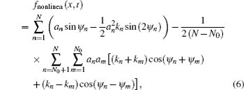
where

n and
m refer to the ordinal numbers of
n-th and the
m-th waves which correspond to the components of short wave and long wave, respectively, and
N0 is the series number of the shortest wavelength in long wave trains. According to the condition of interaction between long wave and short wave,
[18] i.e.,
kN0+1 ≫
kN0, where
n and
m should satisfy the inequalities
n >
N0 and
m≤
N0, where
N0 can be determined by the following criterion:

2.3. One-dimensional nonlinear wave–current coupled fractal sea surface modelRyu et al.[19] developed a numerical wave tank (NWT) with free surface boundary conditions to investigate wave–current interactions and the resulting kinematics. Inspired by their method, we derive a one-dimensional nonlinear wave–current fractal sea surface model in this paper.
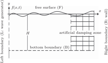
A schematic diagram of the numerical wave tank (NWT) and its boundaries are shown in Fig. 1. The left boundary is between the water and the wave generator. The artificial damping zone closes at the right boundary (wall) of the tank. The wave propagates in the x direction on the free surface. The depth of the water is H, and ξ(x,t) = f (x, t) is the elevation of the water free surface.
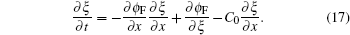
Assuming that the surface current is uniform and C0 is in the x direction, the velocity potential of the sea surface current is

where
C0 is the velocity of the current. Here,
C0 > 0 when the direction of the current is identical to the wave direction, while
C0 < 0 means that the current direction is opposite to the wave direction. Here,
ϕ(
x,
t) represents the unstable wave potential. Equation (
8) satisfies the Laplace equation

The wave should be completely dissipated in the artificial damping zone. According to the boundary conditions on the input boundary (L), the wall (R), and the bottom (B), we have


The kinematic free surface boundary conditions are


where

Sea surface velocity is caused by the motion of free surface water particles; from Eqs. (
13)–(
15), one can obtain
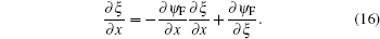
Substituting Eq. (
3) into Eq. (
16) yields
Assuming that the pressure on the free surface is uniform, which is equal to the atmospheric pressure, the Bernoulli equation on the free surface becomes

where
ρ is the water density. Let the atmospheric pressure
Pa be zero and substitute Eq. (
8) into Eq. (
18), then we will have
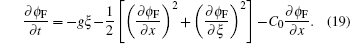
Using initial conditions
ϕ = 0 in the water domain and
ξ = 0 at
t = 0, equation (
19) can be solved as
with
H ≫
ξ in deep sea. Equation (
20) can be simplified into

where
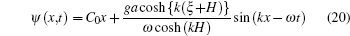
a is the wave amplitude. Therefore, the dispersion relation for the wave–current coupled dynamics in deep water can be written as

and the sea surface can be characterized as
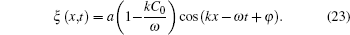
Substituting Eq. (
23) into Eq. (
2), we can obtain the solution for the linear wave–current model as follows:
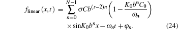
However, the real sea surface is generally nonlinear. Therefore, it is necessary to investigate the nonlinear wave–current model.
Considering nonlinear wave–wave interaction between the long wave and short wave, the nonlinear fractal sea surface model is derived as given in Eq. (6). Using Eqs. (21)–(23) and Eq. (6), one can establish the nonlinear wave–current model as follows:

where
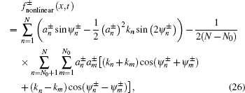
where
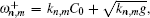
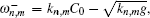 kn,m
kn,m =
K0bn,m,


1 ≤
m≤
N0 and
N0+1≤
n≤
N.
3. Relative error analysisTo estimate the accuracy of our wave–current couple model, wave amplitude is selected to numerically calculate relative error.
Longuet-Higgins and Stewart[18] suggested that the variation in energy of the short wave is caused by the work done by the long wave against the radiation stress of the short wave. According to the Longuet-Higgins and Stewart study, orbital velocities near the free surface have the horizontal component

where
Ψ =
Kx –
ωt +
φ,
h is the depth of water, and the vertical component is

When the wave rides on current
C0, the horizontal component of orbital relative velocity near the free surface can be expressed as

From Eq. (5.16) of Ref. [
19] by Longuet-Higgins and Stewart and Eqs. (
28) and (
29), one can obtain the wave amplitude changes as given below

where
a′ is the effect of the ocean surface current
C0 on the wave amplitude. The above equation becomes

when one considers the wave riding on the surface of deep water.
The relative error er of the difference between the wave amplitude in deep water from our model and that from the analytic solution by Longuet-Higgins MS and Stewart,[18] is
Equation (
32) is used to calculate relative error in the wave amplitude in our model. The root-mean-square (RMS) wave amplitude errors can also easily be obtained based on the relative errors. As an example, figure
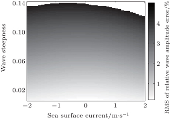
2 shows the relation between sea surface current speed and the RMS relative wave amplitude errors when wave amplitude is 2 m, wave length is 200 m, and sea surface currents range from −2 m·s
−1 to 2 m·s
−1. This range covers most of the ocean surface currents in the world.
Figure 2 shows that the RMS relative wave amplitude error increases with increasing sea surface current magnitude. The maximum RMS of relative error is 5.52% when C0 = 2 m·s−1. The minimum RMS of relative error is 445% when C0 = −0.10 m·s−1. Being relative to the other uncertainties in simulations of ocean waves and wave–current interactions, such as errors in wind fields, unknown physics for wave dissipation, it is acceptable for the model simulation to have a relative error that is less than 10%. Thus, our model presents the results in good agreement with the theoretical results.
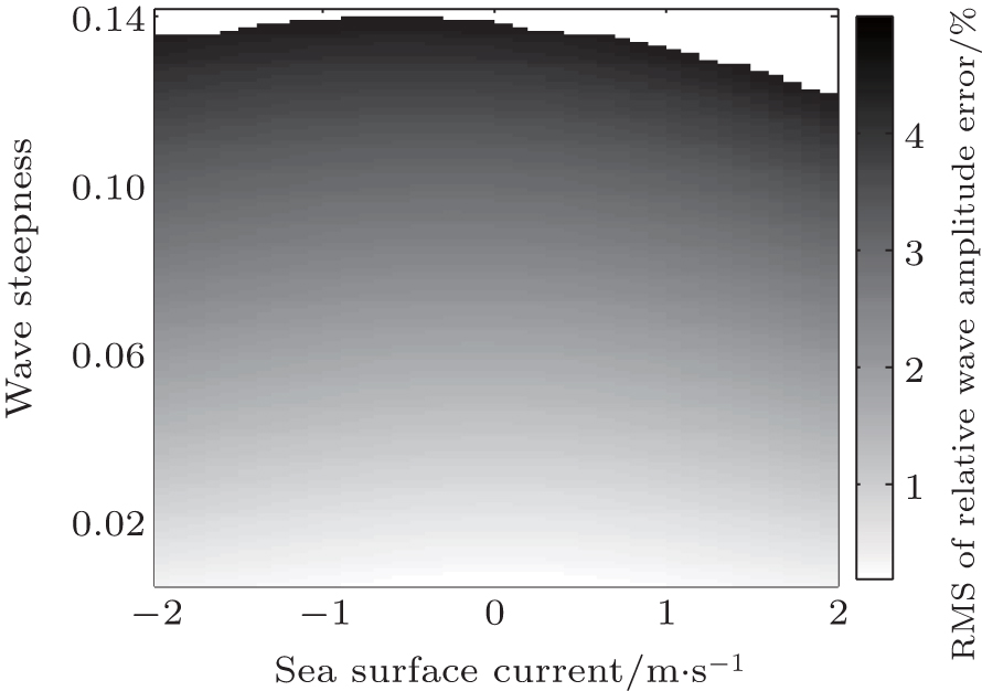
Moreover, the limit of the possible numerical application of our model is studied here. According to Stokes wave theory, the maximum steepness of ocean wave is 0.142. Therefore we let wave steepness increase from 0 to 0.142, and let the velocities of sea surface currents range from −2 m·s−1 to 2 m·s−1. Therefore, the RMS relative wave amplitude error varies with wave steepness and velocity of sea surface current as shown in Fig. 3. The white color in Fig. 3 indicates the case where the RMS relative wave amplitude error is larger than 10%.
Numerical results show that our model can simulate 92% of the case shown in Fig. 3. In other words, the relative error of our model is less than 10% for sea surface current velocity varying over the range from −2 m·s−1 to 2 m·s−1 and for ocean wave steepness less than 0.142.
4. Numerical results and discussionTo find the differences between the current effect on the nonlinear sea surface model and that on its wave–current coupled model, the initial conditions are set to be the same as previous ones, i.e., x = 1 m, λ0 = 200 m, b = 2e/3, σ= 075, s= 13, and N= 25. According to Eq. (7), one can obtain N0= 6. Therefore, all wave components are long waves when N≤6 and the wave components are short waves when N>6.
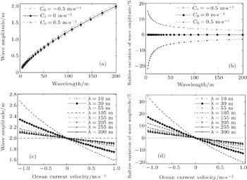
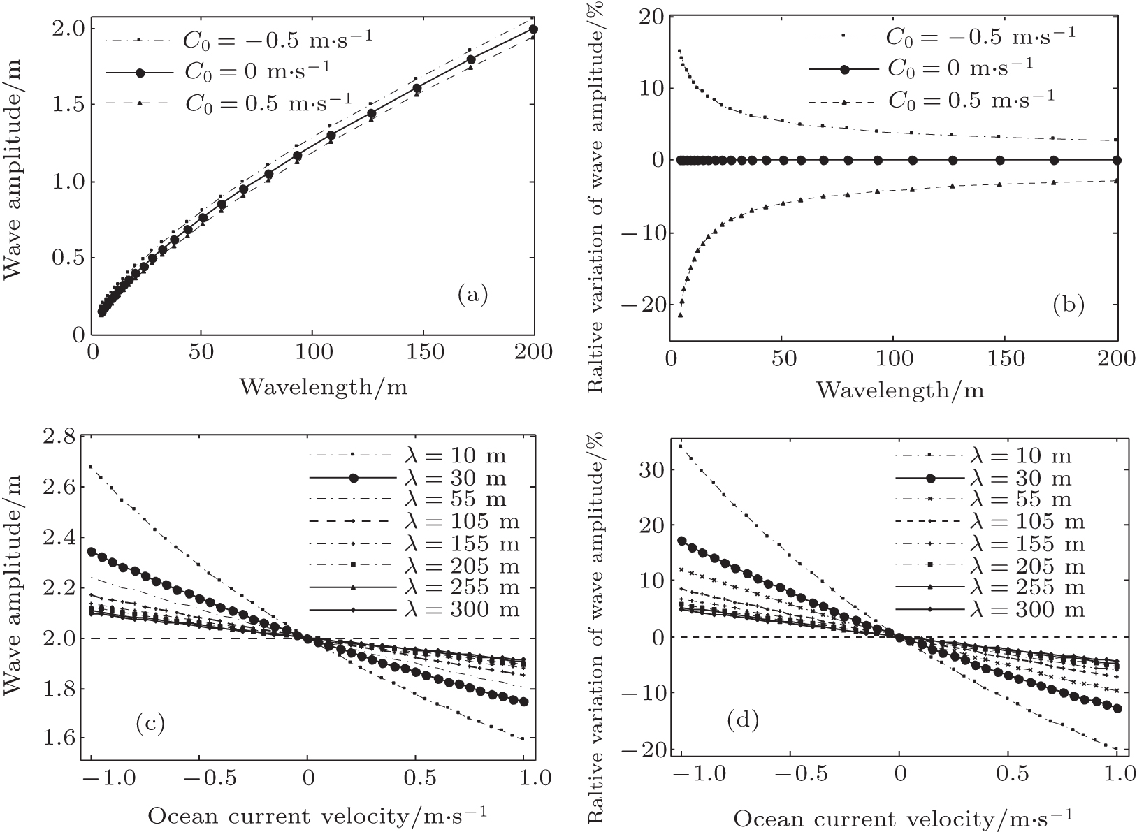
4.1. Effect of current on the wave4.1.1. The effects of currents on wave amplitude and wavelengthThe effect of ocean surface current on wave amplitude is investigated here. Suppose that the velocity of the ocean surface current is positive when the current direction is the same as the wave propagation direction, and negative when the current direction is opposite to the wave propagation direction. Let C0 = ±0.5 m·s−1 and C0 = 0 m·s−1; the effects of current on the wave amplitude for different cases are shown in Fig. 4.
The effects of current on wave amplitude are shown in Fig. 4. Figure 4(a) shows that the wave amplitude increases with increasing wavelength when C0 = 0 m·s−1. Compared with the case where there is no current nor drifting sea surface, wave amplitude decreases when the wave propagates in the same direction as the current direction (for example, C0 = 0.5 m·s−1) whereas wave amplitude increases when the wave propagates in the opposite direction to the current direction (for example, C0 = −0.5 m·s−1). The relative variations of wave amplitude with wavelength corresponding to Fig. 4(a) are shown in Fig. 4(b). From Fig. 4(b), one can find that the effects of current on wave amplitude decrease with increasing wavelength. The effects of current on wave amplitude when wavelengths are less than 50 m are much greater than those when wavelengths are more than 50 m. The maximum relative changes in wave amplitude are 15% (C0 = −0.5 m·s−1) and −21.5% (C0 = 0.5 m·s−1), respectively. Wave amplitudes decrease to 4.3% and −2.9% when wavelength increases to 50 m, respectively. Figure 4(c) shows the variations of wave amplitude with ocean current velocity for different wavelengths. The variations of relative wave amplitudes with ocean current velocity for different wavelengths corresponding to those in Fig. 4(c) are shown in Fig. 4(d). Results show that wave amplitude increases when C0< 0 m·s−1 while wave amplitude decreases when C0> 0 m·s−1 at different wavelengths. In comparison to short waves, the effects of current on long wave amplitude are less than those of short wave.
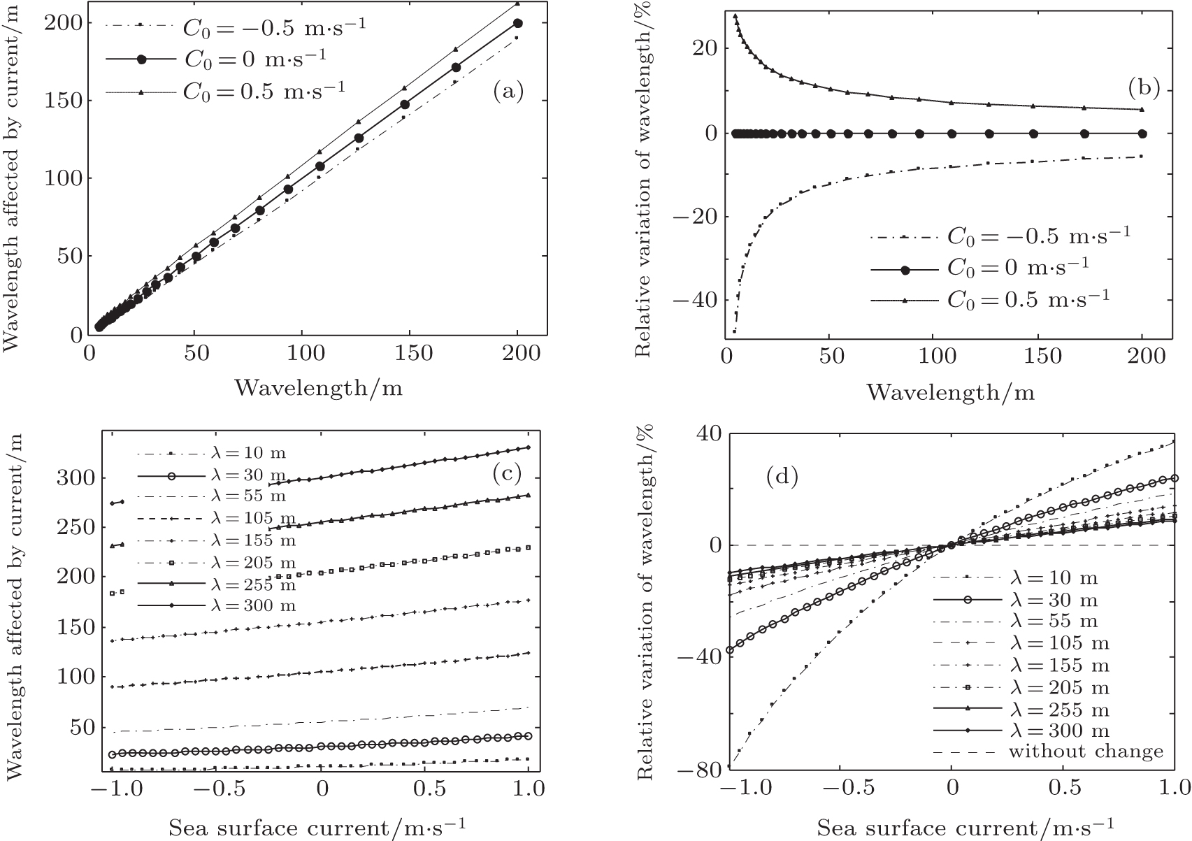
The effects of current on wave wavelength are shown in Fig. 5. Figure 5(a) shows that the wavelength increases when wave propagates in the same direction as the current direction (for example, C0 = 0.5 m·s−1), whereas wavelength decreases when the wave propagates in the opposite direction to the current direction (for example, C0 = −0.5 m·s−1). The relative variations of the wavelength affected by current with wavelength for different current velocities corresponding to those in Fig. 5(a) are shown in Fig. 5(b). From Fig. 5(b), one can find that the effect of current on wavelength decreases with increasing wavelength. The effects of current on wavelength when wavelengths are less than 50 m are much greater than when wavelengths are more than 50 m. The maximum changes of wave amplitude are 27.8% for current C0 = 0.5 m·s−1, and −47.6% for the opposite current C0 = −0.5 m·s−1 respectively. Wavelengths decrease to 10.4% and −12.3% when wavelength increases to 50 m for the parallel and opposite currents, respectively, compared with 5.4% and −5.9% when wavelength increases to 200 m. The changes of wavelength and their relative variation affected by ocean current are shown in Figs. 5(c) and 5(d), respectively. Results show that wavelength is shortened in opposing current and lengthened in collinear current. The overall effect of current on long waves is less than the effect on short waves.
4.1.2. Effects of currents on wave heightsWe now choose the following parameters:

To ensure enough samples, the simulation time interval is set to be
t = [001 s, 3363 s], which is 300 times the dominant period. The simulation time step is 0.01 s in this work. Thus, 336300 samples are obtained.
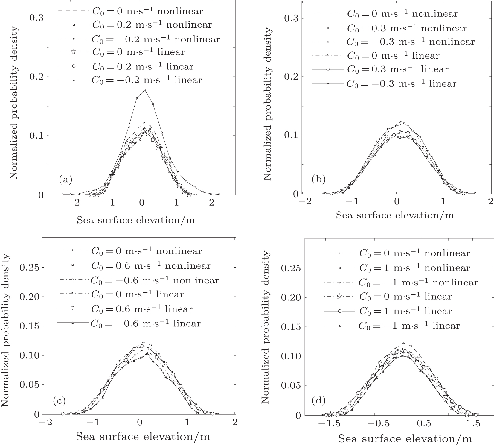
As an example, consider currents of C0 = ±0.6 m·s−1 and C0 = 0 m·s−1 on linear and nonlinear fractal sea surfaces respectively. The wave height evolutions with time are shown in Fig. 6, where figures 6(a)–6(c) show the results of the linear fractal sea surfaces and figures 6(d)–6(f) display the results for the nonlinear fractal sea surface. Different current velocities are included.
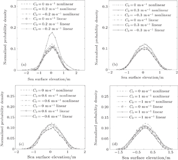
Results in Fig.6 are used to generate statistics and analyze the normalized probability density function (PDF) for wave heights which are shown in Fig. 7, where figures 7(a)–7(d) show the normalized wave height PDFs for the linear and nonlinear fractal sea surface with current velocities of C0 = ±0.2 m·s−1, C0 = ±0.3 m·s−1, C0 = ±0.6 m·s−1, and C0 = ±1 m·s−1, correspondingly. Each of the PDF curves in Fig. 7 has characteristics of a Gaussian curve.
The values of kurtosis (β) and skewness (α) of the wave height PDF of the fractal sea affected by different current velocities in Fig. 7 are listed in Table 1. From Table 1, one can find that PDF distributions of both nonlinear and linear fractal sea surface wave height have positive skewness distributions (α > 0) when C0 = 0 m·s−1, where values of α are changed by current velocity. Here, β is defined as the discrepancy between the fourth order central moment and the kurtosis of the Gaussian distribution (which is 3), i.e., β = Kurtosis – 3. Therefore, β is also affected by currents which can also be seen in Table 1.
Table 1.
Table 1.
 Table 1. Values of kurtosis and skewness of PDF of the fractal sea surface wave height affected by different current velocities. .
| Current velocity C0/m·s−1 |
Linear fractal sea surface |
Nonlinear fractal sea surface |
| β |
α |
β |
α |
| –1.0 |
2.379 |
–0.008 |
2.379 |
0.001 |
| –0.6 |
2.356 |
–0.004 |
2.357 |
–0.002 |
| –0.3 |
2.362 |
–0.001 |
2.363 |
0.002 |
| –0.2 |
2.400 |
–0.001 |
2.402 |
0.002 |
| 0 |
2.411 |
0.001 |
2.467 |
0.005 |
| 0.2 |
2.424 |
–0.004 |
3.459 |
0.097 |
| 0.3 |
2.432 |
–0.009 |
2.509 |
0.014 |
| 0.6 |
2.449 |
0.003 |
2.479 |
0.031 |
| 1.0 |
2.473 |
–0.007 |
2.492 |
0.033 |
| Table 1. Values of kurtosis and skewness of PDF of the fractal sea surface wave height affected by different current velocities. . |
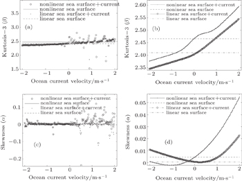
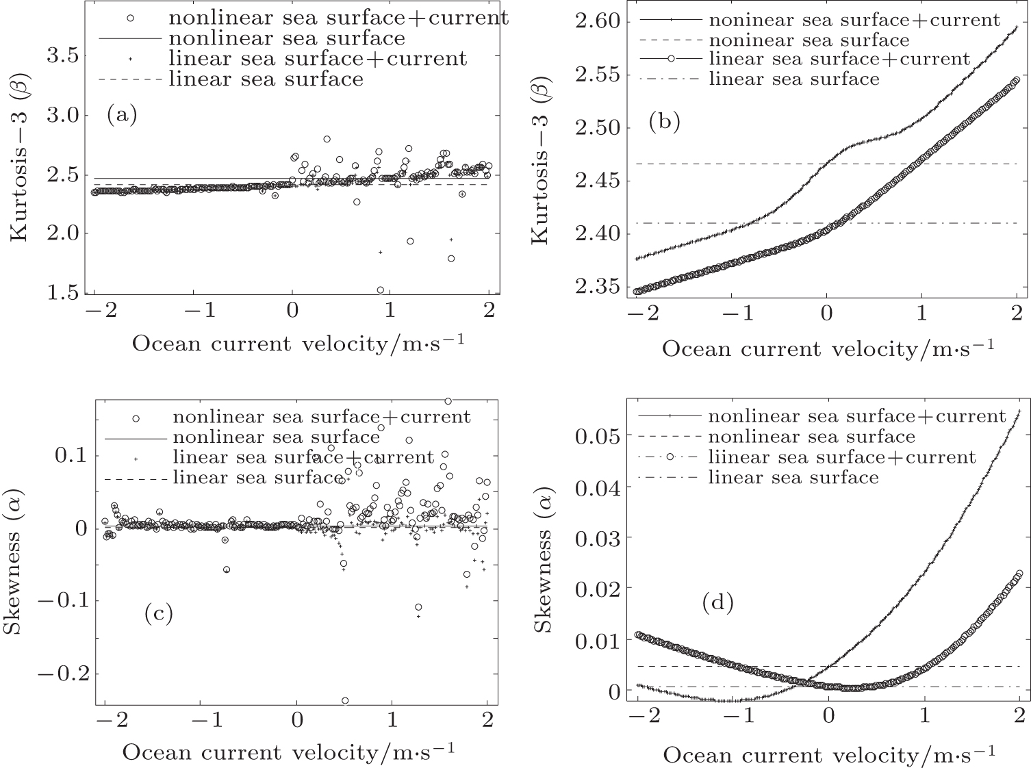
The effective trends of current on kurtosis and skewness of wave height distributions on the linear and nonlinear fractal sea surface are shown in Fig. 8. Ocean current velocity increases from −2 m·s−1 to 2 m·s−1 here. The original β and αdata are shown in Figs. 8(a) and 8(c), respectively. Fitted curves corresponding to Fig. 8(a) and Fig. 8(c) are shown in Figs. 8(b) and 8(d), respectively.
The results in Fig. 8(b) show that for the nonlinear fractal sea surface, the kurtosis of wave height PDF is larger than that of the linear fractal sea surface, under the same currents. Moreover, the kurtosis increases with increasing current velocity. While the skewness interval of the wave height PDF shown in Fig. 8(d) is small, ranging from −0.2 to 0.25, which is much smaller than that of the general PDF, ranging from -3 to 3, the effect of current on the skewness of the wave height PDF is relatively small.
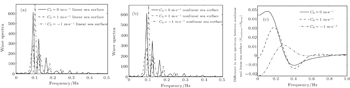
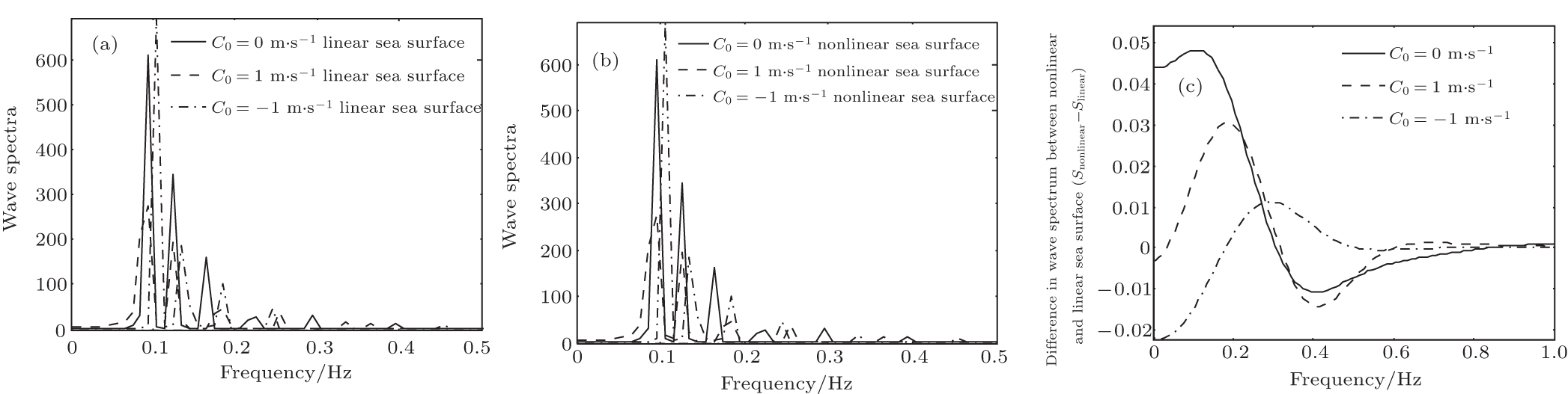
4.2. Effect of current on wave spectrumResults in Fig. 9 show that currents can affect wave spectra of both the linear (Fig. 9(a)) and nonlinear (Fig. 9(b)) fractal sea surface. Differences in wave spectrum between the nonlinear and linear sea surface are shown in Fig. 9(c).
It is shown in both Figs. 9(a) and 9(b) that wave spectrum intensities are strengthened when waves propagate in opposing currents (C0 = −1 m·s−1 in Fig. 9). However, the spectrum peaks shift towards higher frequencies. Therefore, the peak wave lengths must be shortened. Moreover, the wave spectra are weakened in collinear current (C0 = 1 m·s−1 in Fig. 9). In other words, the peak wave lengths are lengthened.
The differences in spectrum between linear and nonlinear fractal sea surfaces, for different current velocities, are shown in Fig. 9(c). The peak spectra for the linear sea surface case, at currents −1 m·s−1 and 1 m·s−1, are 692.6 and 273.7, respectively. The difference is 418.9. The corresponding difference is 418.6 for the nonlinear fractal sea surface. Comparing the effects of current on wave spectrum for linear and nonlinear sea surfaces, the effect of the nonlinearity on the wave spectrum can be ignored.
5. ConclusionsA wave–current coupled model is established in this paper. The model is used to numerically study the effect of the current on the wave.
Numerical simulation results show that the wave amplitude decreases (increases) when the wave propagates in the direction the same as (opposite to) the current direction. Wavelength and wave height kurtosis increase, whereas wave spectrum intensity decreases and shifts towards lower frequencies when current direction is parallel to the ocean wave direction. By comparison, if current direction is opposite to the the wave direction, then wave amplitude increases, wavelength and wave height kurtosis decrease, and spectrum intensity increases and shifts towards higher frequencies. The effect of ocean current is much stronger than that of a nonlinear wave. The kurtosis of the nonlinear fractal ocean surface is larger than that of the linear fractal ocean surface. The effect of current on the skewness of the probability distribution function is negligible.
Our results imply that the ocean wave spectrum distribution is changed by ocean surface currents, which must be reflected in electromagnetic backscattering observations. An electromagnetic backscatter model of the effect of current on fractal sea surface is established in Part 2 of this study, based on the wave–current coupled model presented in this paper (Part 1).


 , Zhao Shang-Zhuo1, 2, Perrie William3, Fang He1, 2, Yu Wen-Jin1, 2, He Yi-Jun1, 2]