Degree distribution of random birth-and-death network with network size decline
[Zhang Xiao-Jun†,  , Yang Hui-Lan]
, Yang Hui-Lan]
|
|


† Corresponding author. E-mail:
Project supported by the National Natural Science Foundation of China (Grant No. 61273015) and the Chinese Scholarship Council.
In this paper, we provide a general method to obtain the exact solutions of the degree distributions for random birth-and-death network (RBDN) with network size decline. First, by stochastic process rules, the steady state transformation equations and steady state degree distribution equations are given in the case of m ≥ 3 and 0 < p < 1/2, then the average degree of network with n nodes is introduced to calculate the degree distributions. Specifically, taking m = 3 for example, we explain the detailed solving process, in which computer simulation is used to verify our degree distribution solutions. In addition, the tail characteristics of the degree distribution are discussed. Our findings suggest that the degree distributions will exhibit Poisson tail property for the declining RBDN.
In the real world, there exist many birth-and-death networks such as the World Wide Web,[1–3] the communication networks,[4–6] the friend relationship networks,[7–10] and the food chain networks,[11–13] in which nodes may enter or exit at any time. For these kinds of evolving networks, the degree distribution is always one of the most important statistical properties.[14–31] Several methods have been proposed to calculate their degree distributions like the first-order partial-differential equation method,[14] the mean-field approach,[15,16] the rate equation approach,[17–20,30] and the master-equation approach.[31] While these approaches aim at the networks whose sizes keep growing or remain unchanged at each time step, Zhang et al. put forward the stochastic-process-rules (SPR)-based Markov chain method to solve the degree distributions of evolving networks in which the network size may increase or decrease at each time step.[21]
Furthermore, a random birth-and-death network model (RBDN) is considered,[27] in which at each time step, a new node is added into the network with probability p (0 < p < 1) and connected with m old nodes uniformly, or an existing node is deleted from the network with the probability q = 1 − p. For 0 < p < 1/2, since m is a critical parameter for the degree distributions, solution methods may vary for different values of m. Zhang et al. only considered special cases, i.e., m = 1 and 2.[27] In this paper, a general approach is proposed for solving the degree distributions of RBDN with network size decline in the case of m ≥ 3. Taking m = 3 for example, we provide the exact solutions of the degree distributions for RBDN. Our findings indicate that the tail of the degree distribution for the declining RBDN is subject to Poisson tail.
The rest of this paper is structured as follows: Section 2 gives the RBDN model with 0 < p < 1/2 and its steady-state equations; Section 3 provides the method of solving degree distribution of RBDN with 0 < p < 1/2; Section 4 further discusses the tail characteristics of the degree distribution; Section 5 concludes the paper.
Consider the RBDN model:[27]
By the above evolving roles, the network size of the RBDN is always fluctuating in the evolving process. In particular, in the limit t → + ∞, the distribution of the network size follows geometric distributions.[27]
Using SPR,[21] we use (n,k) to describe the state of node v, where n is the number of nodes in the network that contains v, and k is the degree of node v. Let NK(t) denote the state of node v at time t, the stochastic process {NK(t), t ≥ 0} is an ergodic aperiodic homogeneous Markov chain with the state space E = {(n,k),n ≥ 1,0 ≤ k ≤ n − 1}.
Let 


Let K be the steady state degree distribution,[15,30,31] and Π (k) be the probability distribution of K, then we will have

Combining Eq. (
Let N(t) be the number of nodes in RBDN at time t, N(0) = m + 1, N the steady state network size, and ΠN(n) the probability distribution of N, then we will have

As shown in Eq. (

To obtain Π(i,k), 


Once Π(i,k) is obtained, the probability generating function approach can be employed for Eq. (


To solve Π (k), let the probability generating function be


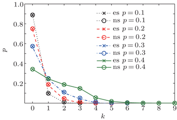
Figure
 | Fig. 1. Comparisons between exact solution and numerical solution (t = 104) of degree distribution of RBDN for p < 1/2, m = 3. |
By Eq. (

Let


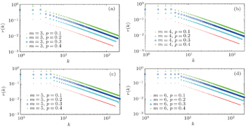
Figure
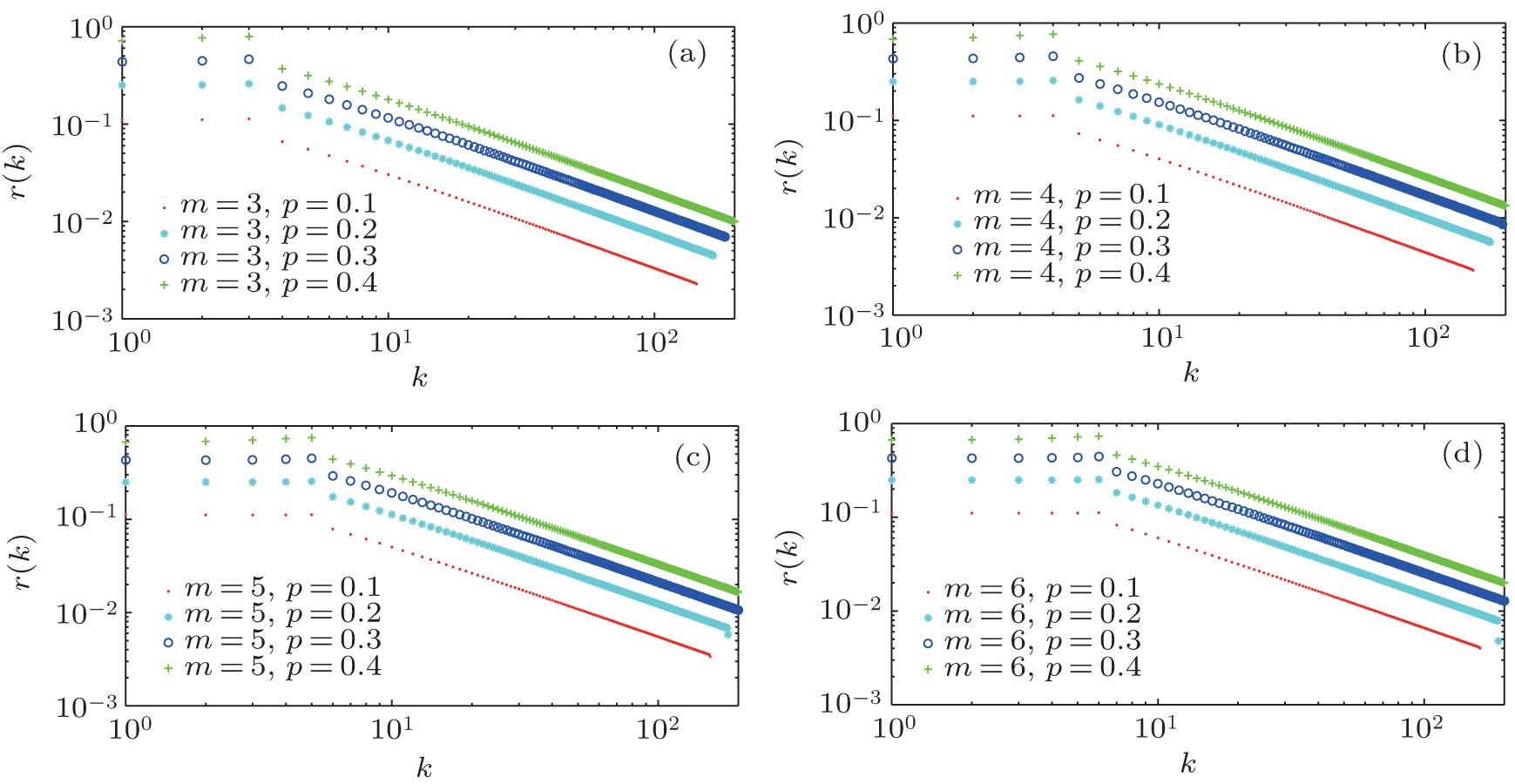 | Fig. 2. Poisson tails of RBDN with 0 < p < 1/2. |
In this paper, we provide a general approach to obtaining the exact solutions of the degree distributions for RBDN in the case of 0 < p < 1/ 2, m ≥ 3. Specifically, taking m = 3 for example, we explain the detailed solving process and computer simulation is used to verify our degree distribution solutions. In addition, the characteristics of the degree distribution are discussed. Our findings suggest that the degree distributions will exhibit Poisson tail property for the declining RBDN.
| 1 | |
| 2 | |
| 3 | |
| 4 | |
| 5 | |
| 6 | |
| 7 | |
| 8 | |
| 9 | |
| 10 | |
| 11 | |
| 12 | |
| 13 | |
| 14 | |
| 15 | |
| 16 | |
| 17 | |
| 18 | |
| 19 | |
| 20 | |
| 21 | |
| 22 | |
| 23 | |
| 24 | |
| 25 | |
| 26 | |
| 27 | |
| 28 | |
| 29 | |
| 30 | |
| 31 |