Nonlocal symmetry and exact solutions of the (2+1)-dimensional modified Bogoyavlenskii–Schiff equation
Huang Li-Li, Chen Yong†,
Shanghai Key Laboratory of Trustworthy Computing, East China Normal University, Shanghai 200062, China


† Corresponding author. E-mail: ychen@sei.ecnu.edu.cn

Project supported by the Global Change Research Program of China (Grant No. 2015CB953904), the National Natural Science Foundation of China (Grant Nos. 11275072 and 11435005), the Doctoral Program of Higher Education of China (Grant No. 20120076110024), the Network Information Physics Calculation of Basic Research Innovation Research Group of China (Grant No. 61321064), and the Fund from Shanghai Collaborative Innovation Center of Trustworthy Software for Internet of Things (Grant No. ZF1213).

Abstract
Abstract

In this paper, the truncated Painlevé analysis, nonlocal symmetry, Bäcklund transformation of the (2+1)-dimensional modified Bogoyavlenskii–Schiff equation are presented. Then the nonlocal symmetry is localized to the corresponding nonlocal group by the prolonged system. In addition, the (2+1)-dimensional modified Bogoyavlenskii–Schiff is proved consistent Riccati expansion (CRE) solvable. As a result, the soliton–cnoidal wave interaction solutions of the equation are explicitly given, which are difficult to find by other traditional methods. Moreover figures are given out to show the properties of the explicit analytic interaction solutions.

1. Introduction

Soliton equations connect rich histories of exactly solvable systems constructed in mathematics, fluid physics, micro-physics, cosmology, field theory, etc. To explain some physical phenomenon further, it becomes more and more important to seek exact solutions and interactions among solutions of nonlinear wave solutions. It is well known that there are many ways to obtain exact solutions of soliton equations, such as the Inverse Scattering transformation (IST),[1] Bäcklund transformation (BT),[2] Darboux transformation (DT),[3,4] Hirota bilinear method,[5] Painlevé method,[6,7] Lie symmetry method,[810] and so on. For a given nonlinear system, the Lie symmetry method proposed by Sophus Lie[11,12] during the nineteenth century is a standard method to find the corresponding Lie point symmetry algebras and groups.

The nonlocal symmetries are connected with integrable models and they enlarge the class of symmetries, therefore, to search for nonlocal symmetries of the nonlinear systems is an interesting work. Akhatov and Gazizov[13] provided a method for constructing nonlocal symmetries of differential equations based on the Lie–Bäcklund theory. Galas[14] obtained the nonlocal Lie–Bäcklund symmetries by introducing the pesudo-potentials as an auxiliary system. Guthrie[15] got nonlocal symmetries with the help of a recursion operator. Bluman[16] introduced the concept of potential symmetry for a differential system by writing the given system in a conserved form. Lou et al.[1719] have made some efforts to obtain infinitely many nonlocal symmetries by inverse recursion operators, the conformal–invariant form (Schwartz form), and Darboux transformation. More recently, Lou, Hu, and Chen[2022] obtained nonlocal symmetries that were related to the Darboux transformation with the Lax pair and Bäcklund transformation. Xin and Chen[23] gave a systemic method to find the nonlocal symmetry of nonlinear evolution equation and improved previous methods to avoid missing some important results such as integral terms or high-order derivative terms of nonlocal variables in the symmetries. In recent years, it was found that Painlevé analysis can be used to obtain nonlocal symmetries. The type of nonlocal symmetry related to the truncated Painlevé expansion is just the residual of the expansion with respect to singular manifold, and is also called residual symmetry.[2428] The localization of this type of residual symmetry seems more easily performed than that coming from DT and BT. In order to develop some types of relatively simple and understandable methods to construct exact solutions, Lou proposed a consistent Riccati expansion (CRE) method to identify CRE solvable systems in Ref. [29]. A system is defined to be CRE solvable if it has a CRE. It has been revealed that many similar interaction solutions between a soliton and a cnoidal wave were found in various CRE solvable systems. By this method, recent studies[3038] have found a lot of interaction solutions in many nonlinear equations.

In the present paper, we focus on investigating the nonlocal symmetry, prolonged system, Bäcklund transformation, CRE solvability, and the exact interaction solutions of the following (2+1)-dimensional modified Bogoyavlenskii–Schiff (mBS) equation[3943]

where subscript means a partial derivative such as ut = ∂u/∂t, uxy = 2u/∂x∂y, and

This equation can be derived by the following CD-type (2+1)-dimensional breaking soliton equation[4446]

with a Miura transformation,

It is obvious that if y = x the equation becomes an mKdV equation,

which is widely researched by several authors. In order to treat the integral appearing in the equation, equation (1) is then rewritten as

As equation (2) is a typical breaking soliton equation to describe the (2+1)-dimensional interaction of a Riemann wave propagating along the y axis with a long wave along the x axis and equation (4) may present the wave propagation of the bound particle, sound wave, and thermal pulse, equation (1) must have abundant physical phenomena. But little attention has been paid to this equation, except Refs. [39]– [43], where the Lax pair and soliton solutions are presented. Therefore, finding more types of solutions of Eq. (1) is of interest to understand the equation fully.

This paper is arranged as follows. In Section 2, the non-auto Bäcklund transformation and nonlocal symmetry of the (2+1)-dimensional modified mBS equation are obtained by making use of the truncated Painlevé expansion approach, then the nonlocal symmetry is localized by introducing another three dependent variables and the corresponding nonlocal transformation group is found. In Section 3, the (2+1)-dimensional modified mBS equation is verified to be consistent Riccati expansion solvable and the soliton–cnoidal wave solutions are constructed. The last section contains a summary and discussion.

2. The nonlocal symmetry from the truncated Painlevé expansion

For the (2+1)-dimensional mBS equation (5), there exists a truncated Painlevé expansion

with u0,u1,v0,v1,v2,ϕ being the functions of x, y, and t, the function ϕ(x,y,t) = 0 is the equation of singularity manifold.

Substituting Eq. (6) into Eq. (5) and balancing all the coefficients of different powers of ϕ, we can get

and the (2+1)-dimensional mBS equation (5) is successfully satisfying the following Schwarzian form

Here, we denote

where P is the usual Schwarzian variables, S is the Schwarzian derivative and both invariants under the Möbious transformation, i.e.,

If we take a special case a = 0, b = c = 1, d = ɛ, then equation (10) can be rewritten as

which means equation (8) possesses the point symmetry[24]

From the standard truncated Painlevé expansion (6), we have the following non-auto-Bäcklund transformation theorem of Eq. (5).

Theorem 1 (non-auto-BT theorem) If the function ϕ satisfies Eq. (8), then,

is a non-auto BT between ϕ and the solution u,v of the (2+1)-dimensional mBS equation (5).

One knows that the symmetry equations for Eq. (5) read

where σu and σv denote the symmetries of u and v, respectively. From the truncated Painlevé expansion (6) and the Theorem 1, a new nonlocal symmetry of Eq. (5) is presented and studied as follows.

Theorem 2 The equation (5) has the nonlocal symmetry given by

where u,v and ϕ satisfy the non-auto BT (12).

Proof The nonlocal symmetries (14) are residual of the singularity manifold ϕ. The nonlocal symmetries (14) will also be obtained with substituting the Möbious transformation symmetry σϕ into the linearized equation (7).

To find out the group of the nonlocal symmetry (14)

we have to solve the following initial value problem

with ɛ being the infinitesimal parameter.

However, since it is difficult to solve Eqs. (15) for (ɛ) and (ɛ) due to the intrusion of the function and its differentiations, we introduce new variables to eliminate the space derivatives of

Now the nonlocal symmetry (14) of the original equation (5) becomes a Lie point symmetry of the prolonged system (5), (12), and (16), saying

The result (17) indicates that the nonlocal symmetries (14) are localized in the properly prolonged systems (5), (12), and (16) with the Lie point symmetry vector

In other words, the symmetries related to the truncated Painlevé expansion are just a special Lie point symmetry of the prolonged system.

Now we have obtained the localized nonlocal symmetries, an interesting question is what kind of finite transformation would correspond to the Lie point symmetry (18). We have the following theorem.

Theorem 3 If {u,v,ϕ,f,g,h} is a solution of the prolonged systems (5), (12), and (16), then {,,,,,} is given by

with arbitrary group parameter ɛ.

Proof Using Lie’s first theorem on vector (18) with the corresponding initial condition

One can easily obtain the solutions of the above equations given in Theorem 3, thus the theorem is proved.

Actually, the above group transformation is equivalent to the truncated Painlevé expansion (6) since the singularity manifold equations (5), (12), and (16) are form-invariant under the transformation

with ɛ fϕx, ɛgϕy, ɛhϕxy.

Next let us study Lie point symmetries of the prolonged systems instead of the single Eq. (5). According to the classical Lie point symmetry method, the Lie point symmetries for the whole prolonged systems possess the form

where X,Y,T,U,V,Φ,F,G,H are functions of x, y, t, u, v, ϕ, f, g, h, which means that the prolonged systems (5), (12), and (16) are invariant under the transformations

with the infinitesimal parameter ɛ.

The symmetries σk (k = u,v,ϕ,f,g,h) are defined as the solution of the linearized equations of the prolonged systems (5), (12), and (16).

We substitute the expressions (19) into the symmetry equations (21) and collect the coefficients of the independent partial derivatives of dependent variables u, v, ϕ, f, g, h. Then we obtain a system of overdetermined linear equations for the infinitesimals X,Y, T,U, v,Φ, F,G, H, which can be easily given by solving the determining equations

where f1f1(t) is an arbitrary function of t,

are arbitrary functions of y and c1,c2,c3, and c4 are arbitrary constants. When

and f2 = −2, the obtained symmetry is just Eq. (17), and when f2 = 0, the related symmetry is only the general Lie point symmetry of the original equation (5). To obtain more group invariant solutions, we would like to solve the symmetry constraint condition σk = 0 defined by Eq. (19) with Eq. (22), which is equivalent to solving the following characteristic equations

To solve the characteristic equations, one special case is listed in the following.

Without loss of generality, we assume c1 = c2 = c3 = 0, c4 = 1, f1 = 1/c5,f2 = c6,f3 = c7, and f4 = c8. For simplicity, we introduce . We find the similarity solutions after solving out the characteristic equations (23)

where

are the group-invariant functions while ξ = y and η = tc5x are the similarity variables. Substituting Eqs. (24) into the prolonged systems (5), (12), and (16), the invariant functions F1, F2, F3, F4, F5, and F6 satisfy the reduction systems

in the above equations, F1 satisfies the following reduction equation

It is obvious that once the solutions F1 are solved out with Eq. (26), the solutions for F2, F3, F4, F5, and F6 can be solved out directly from Eq. (25). So the explicit solutions for the (2+1)-dimensional modified mBS equation (5) are immediately obtained by substituting F1, F2, F3, F4, F5, and F6 into Eq. (24).

3. CRE solvable and soliton–cnoidal waves solution
3.1. CRE solvable

For the (2+1)-dimensional mBS equation (5), we aim to look for its truncated Painlevé expansion solution in the following possible form

where R(w) is a solution of the Riccati equation

with b0,b1,b2 being arbitrary constants. By vanishing all the coefficients of the power of R(w) after substituting Eq. (28) with Eq. (27) into Eq. (5), we have nine over-determined equations for only six undetermined functions u0, u1, v0, v1, v2, and w, it is fortunate that the overdetermined system may be consistent, thus we obtain

and the function w must satisfy

where

From above discussion, it is shown that equation (5) really has the truncated Painlevé expansion solution related to the Riccati equation (28). At this point, we call the expansion (27) a consistent Riccati expansion (CRE) and the (2+1)-dimensional mBS equation is CRE solvable.[29]

In summary, we have the following theorem:

Theorem 4 If w is a solution of

then,

is a solution of Eq. (5), with RR(w) being a solution of the Riccati equation (28).

3.2. Soliton–cnoidal wave interaction solutions

Obviously, the Riccati equation (28) has a special solution R(w) = tanh(w), while the truncated Painlevé expansion solution (27) becomes

where u0, u1, v0, v1, v2, and w are determined by Eqs. (28), (29), and (30).

We know the solution (34) is just consistent with Theorem 4. As consistent tanh-function expansion (CTE) (34) is a special case of CRE, it is quite clear that a CRE solvable system must be CTE solvable, and vice versa. If a system is CTE solvable, some important interaction solitary wave solutions can be constructed directly. In order to say the relation clearly, we give out the following Bäcklund transformation.

Theorem 5 (BT) If w is a solution of Eq. (30) with δ = 4, then

is a solution of Eq. (5), where {u0,v0} is determined by Eq. (29) with b0 = 1, b1 = 0, b2 = −1, δ = 4.

In order to obtain the solution of Eq. (5), we consider w in the form

where g is a function of x,y and t. It will lead to the interaction solutions between a soliton and other waves. By means of Theorem 5, some nontrivial solutions of (2+1)-dimensional mBS equation can be obtained from some quite trivial solutions of Eq. (23), which are listed as follows.

Case 1 In Eq. (30), we take a trivial solution for w, saying

with k, l, d, and c being arbitrary constants. Then substituting Eq. (36) into Theorem 5 yields the following kink soliton and ring soliton solution of the (2+1)-dimensional mBS equation (5)

Case 2 To find out the interaction solutions between soliton and cnoidal periodic wave, let

where W1W1(X) = WX satisfies

with a0, a1, a2, a3, and a4 being constants. Substituting Eq. (39) with Eq. (40) into Theorem 4, we have the following relations

which leads to the following explicit solutions of Eq. (5) in the form of

It is known that an equation by the definition of the elliptic functions can be written out in terms of Jacobi elliptic functions. The formula (42) exhibits the interactions between soliton and abundant cnoidal periodic waves. To show these soliton–cnoidal waves more intuitively, we just take a simple solution of Eq. (40) as

where sn(mX,n) is the usual Jacobi elliptic sine function. The modulus n of the Jacobi elliptic function satisfies: 0 ≤ n ≤ 1. When n → 1, sn(ξ) degenerate as hyperbolic function tanh(ξ), when n → 0, sn(ξ) degenerates as a trigonometric function sin(ξ). Substituting Eq. (43) with Eq. (41) into Eq. (40) and setting the coefficients of cn(ξ), dn(ξ), sn(ξ) equal zero, yields

Hence, one kind of soliton–cnoidal wave solution is obtained by taking Eq. (43) and

with the parameter requirement (44) into the general solution (42).

The solution given in Eq. (42) with Eq. (41) denotes the analytic interaction solution between the soliton and the cnoidal periodic wave. In Fig. 1, we plot the interaction solution of the potential u when the value of the Jacobi elliptic function modulus n ≠ 1. In Fig .2, we plot the interaction solution of the potential v when the value of the Jacobi elliptic function modulus n ≠ 1. This kind of solution can be easily applicable to the analysis of interesting physical phenomenon. In fact, there are plentiful solitary waves and cnoidal periodic waves in the real physics world.

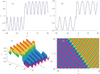
Fig. 1. The first type of soliton–cnoidal wave interaction solution for u with the parameters m = 1, n = 1/2, k2 = 1, μ0 = 1, and μ1 = 1/4: (a) one-dimensional image at x = 0, t = 2; (b) one-dimensional image at x = 0, y = 2; (c) the three-dimensional plot; (d) overhead view for u at t = 0.
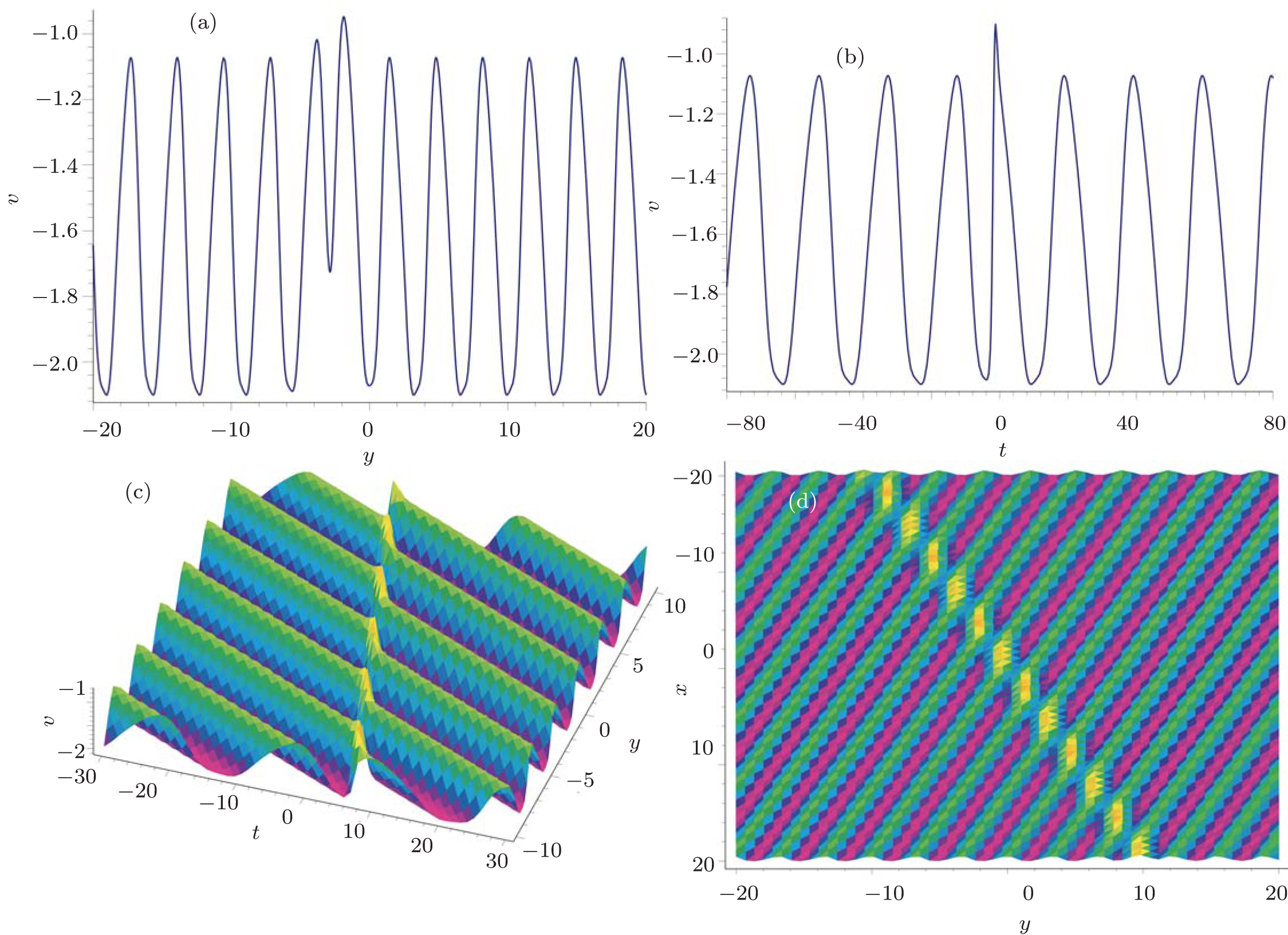
Fig. 2. The first type of soliton–cnoidal wave interaction solution for v with the parameters m = 1, n = 1/2, k2 = 1, μ0 = 1, and μ1 = 1/4: (a) one-dimensional image at x = 0, t = 2; (b) one-dimensional image at x = 0, y = 2; (c) the three-dimensional plot; (d) overhead view for v at t = 0.
4. Summary and discussion

In summary, the (2+1)-dimensional mBS equation is investigated by using the truncated Painlevé analysis. The nonlocal symmetries, Bäcklund transformations and CRE solvable of the equation are found. Then by means of the CRE method, the soliton–cnoidal wave solutions of the (2+1)-dimensional mBS equation are obtained. By a special form of CRE, i.e., the consistent tanh-function expansion (CTE), kink soliton+cnoidal periodic wave solution and ring soliton+cnoidal periodic wave solution are explicitly expressed by the Jacobi elliptic functions and the corresponding elliptic integral. The interactions between solitons and cnoidal periodic waves display some interesting and physical phenomena. The CRE method used here can be developed to find other kinds of solutions and integrable models. It can also be used to find interaction solutions among different kinds of nonlinear waves. The CRE method did provide us with the result which is quite nontrivial and difficult to be obtained by other traditional approaches.

In addition, the generalized mKdV equation has been investigated in many aspects, but numerical methods relevant to the (2+1)-dimensional mBS equation have been reported little in the current articles. So uncovering more integrable properties of the equation, such as the Darboux transformation, Hamiltonian structure and the conservation, are interesting and meaningful work. The details on the CRE method and other methods to solve interaction solutions among different kinds of nonlinear waves and the investigation of other integrability properties such as Hamiltonian structure and generalized nonlocal symmetry of the (2+1)-dimensional mBS equation deserves further study.

Reference
1Ablowitz M JClarkson P A1991Solitons, Nonlinear Evolution Equations and Inverse ScatteringCambridgeCambridge University Press
2Rogers CSchief W K2002Bäcklund and Darboux Transformations: Geometry and Modern Applications in Soliton TheoryCambridgeCambridge University Press
3Matveev V BSalle M A1991Darboux Transformations and SolitonsBerlinSpringer
4Gu C HHu H SZhou Z X1999Darboux Transformation in Soliton Theory and Its Geometric ApplicationsShanghaiShanghai Scientific and Technical Publishers
5Hirota R2004The Direct Method in Soliton TheoryCambridgeCambridge University Press
6Weiss JTabor MCarnevale G1983J. Math. Phys.24522
7Weiss J1983J. Math. Phys.241405
8Bluman G WCole J D1969J. Math. Mech.181025
9Olver P JRosenau P1986Phys. Lett. A114107
10Chen YDong Z Z2009Nonlinear Anal.71e810
11Olver P J1986Application of Lie Group to Differential EquationNew YorkSpringer
12Bluman G WAnco S C2002Symmetry and Integration Methods for Differential EquationsNew YorkSpringer
13Akhatov I SGazizov R K1991J. Math. Sci.551401
14Galas F1992J. Phys. A: Math. Gen.25L981
15Guthrie G A1993J. Phys. A: Math. Gen.26L905
16Bluman G WCheviakov A FAnco S C2010Applications of Symmetry Methods to Partial Differential EquationsNew YorkSpringer
17Lou S Y1993Phys. Lett. B302261
18Lou S Y1997J. Phys. A: Math. Gen.304803
19Lou S YHu X B1997J. Phys. A: Math. Gen.30L95
20Hu X RLou S YChen Y2012Phys. Rev. E85056607
21Lou S YHu X RChen Y2012J. Phys. A: Math. Theor.45155209
22Hu X RChen Y2015Chin. Phys. B24030201
23Xin X PChen Y2013Chin. Phys. Lett.30100202
24Lou S Y2013arXiv:1308.1140
25Gao X NLou S YTang X Y2013JHEP05029
26Yu JRen BLiu X Z2015Chin. Phys. B24030202
27Ren BYang J RZeng B Q2015Chin. Phys. B24010202
28Yang J RRen BYu J2015Chin. Phys. B24010203
29Lou S Y2015Studies in Applied Mathematics134372
30Hu X RChen Y2015Z. Naturforsch. A70729
31Ren BLiu X ZLiu P2015Commun. Theor. Phys.63125
32Ren B2015Phys. Scr.90065206
33Hu X RLi Y Q2016Appl. Math. Lett.5120
34Hu X RChen Y2015Chin. Phys. B24090203
35Wang QChen YZhang H Q2005Chaos, Solitons and Fractals251019
36Wang Y HWang H2014Phys. Scr.89125203
37Yu W FLou S YYu J2014Chin. Phys. Lett.31070203
38Yu G XRuan S QYu J etc.2015Chin. Phys. B24060201
39Toda KYu S JFukuyama T1998J. Phys. A: Math. Gen.3110181
40Toda KYu S JFukuyama T1999Rep. Math. Phys.44247
41Yu S JToda K2000J. Nonlinear Math. Phys.71
42Yu S JToda KFukuyama T2008arXiv:9802005
43Wazwaz A M2012Commun. Nonlinear Sci. Numer. Simul.171500
44Calogero FDegasperis A1976Nuovo Cimento B32201
45Calogero FDegasperis A1977Nuovo Cimento B391
46Fan E GChow K W2011J. Math. Phys.52023504