1. IntroductionThe order (defined as the number of nodes) of many scale-free networks grows over time, e.g., social networks, airport networks, and Internet topologies.[1] Thus, it is inevitable to compare networks with different orders for the study of these evolving systems. Network comparison has been widely used for the classification and similarity analysis of diverse networks. Specifically, the comparison of networks with different orders strongly depends on the stability features of the evolving systems. This paper focuses on the stability analysis of a spectral graph feature of scale-free evolving systems, i.e., the weighted spectral distribution (WSD).
Graph spectra incorporate all eigenvalues of graph matrices, including adjacency and normalized Laplacian matrices. The natural connectivity is a spectral graph feature defined on the adjacency spectrum.[2] Moreover, Wu et al.[3] rigorously demonstrated that the feature is asymptotically independent of the order of regular graphs in which each node has an identical expected degree. However, our recent work[4,5] found numerically that the stability of the natural connectivity does not work in scale-free networks. The WSD is another spectral graph feature defined on the normalized Laplacian spectrum that strongly corresponds to the distribution of random N-cycles in a network.[6] Fay et al.[7] designed a calculation algorithm for the WSD using Sylvester’s law of inertia which is restricted to networks with less than 30000 nodes. Using 4-cycle structures, Jiao et al.[4] proposed a fast algorithm by which the WSD can be accurately calculated in scale-free networks with more than millions of nodes. The WSD captures the local connectivity of diverse networks.[8,9] Additionally, Jiao et al.[5] numerically observed that the WSD increases sublinearly with the network order in a stochastic scale-free network model. However, the stochastic models are not suitable for the rigorous analysis of the WSD’s stability since it is impossible to derive the WSD’s precise formula in these models. Therefore, there is a need to rigorously investigate the stability of the WSD for better understanding the performance of the spectral graph feature in evolving scale-free networks.
In contrast to stochastic models, deterministic models help us to understand the construction rules embedded in randomized structures and allow for rigorous computation of many graph features, e.g., clustering coefficients, diameter, betweenness, path length, and mean first-passage time.[10–20] The primary deterministic scale-free model was proposed by Barabasi et al.[19] However, this model lacks the small-world effect that exists in most real networks, i.e., its clustering coefficient is too small while the average length path remains relatively large. To remedy this weakness, Chen et al.[20] constructed a pseudo tree-like (PTL) deterministic model having both the small-world and the scale-free characteristics. Moreover, in Chen’s model,[20] the distribution of clustering coefficients C(k) with respect to degree k has the power-law form C(k) ∝ k−1 which exists in most hierarchical systems.[21] Therefore, our contribution includes the rigorous analysis of the WSD’s stability using Chen’s deterministic model.
2. Background2.1. WSDLet G = (V,E) be a simple and undirected graph, where V and E are the node set and the edge set, respectively. Let dv be the degree of a node v in graph G. Then, the normalized Laplacian matrix of graph G can be expressed as[6]
All eigenvalues of matrix
L(
G) (i.e., 0 =
λ1 ≤ ⋯ ≤
λn ≤ 2) form the normalized Laplacian spectrum. The WSD is defined as follows:
[7]

Additionally, the WSD counts the sum over all
N-cycles in graph
G[7]

where
C =
u1u2⋯
uN is all
N-cycles in graph
G. The parameter
N represents many graph properties. One important property is the number of 4-cycles. For a graph of its density, it is quasi-random.
[22,23] In general, the sum over the 4-cycles represents the quasi-randomness of the graph in a non-regular case.
[22,23] Therefore, four is considered to be the suitable value of the parameter
N.
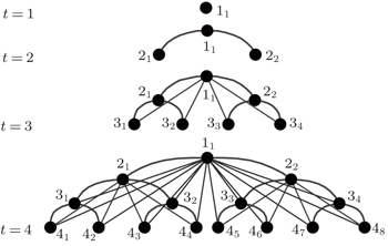
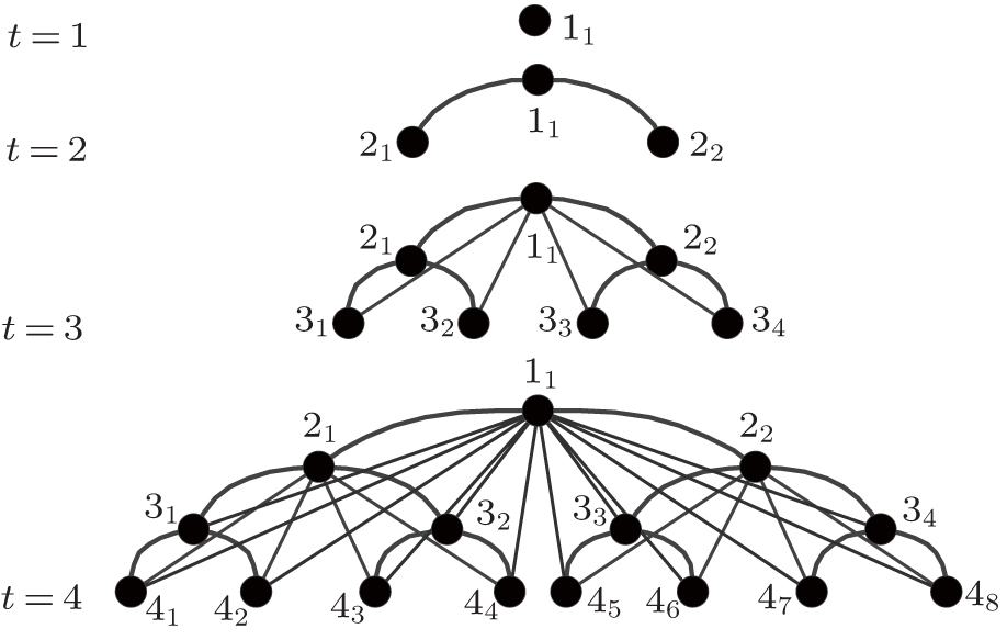
[4–6] 2.2. Pseudo tree-like modelLet Tn+1 denote the n + 1 hierarchical-level graph generated by the PTL model. Specifically, Tn+1 is generated recursively with level t increased from 1 to n + 1 as follows (Fig. 1).[20]
At t = 1, start with a single node 11, which is the main root of the whole network.
At t = 2, two leaf nodes 21 and 22 are added and connected to the main root 11.
At t = 3, four leaf nodes 31–34 are added and each node 3j (1 ≤ j ≤ 4) is connected to the main root 11 and the subordinate root 21 (for j = 1, 2) or 22 (for j = 3, 4).
In general, at level t ∈ {1,2,…,n + 1}, 2t−1 leaf nodes tj (1 ≤ j ≤ 2t−1) are added and each node tj is connected to its t − 1 roots (t − k)⌈j/2k⌉ (k = 1,2,…,t − 1), where ⌈x⌉ rounds the value of x to the nearest integer towards infinity.
Chen et al.[20] demonstrated that the PTL model has the scale-free, the small-world, and the hierarchical characteristics of most complex networks.
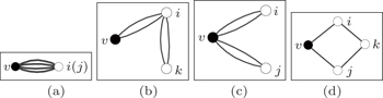
3. Precise formula of the WSD in Tn+1Equations (2) and (3) show that the WSD counts the sum of the products of degree reciprocals embedded in all N-cycles (N = 4 is commonly selected) of graph G. For each node v ∈ V, let N(v) = {1,2,…,r} denote the set of neighbors of node v and  denote the set of neighbors of node i ∈ {1,2, …,r}. Let C(i, j) = {v,c1,c2, …,ctij} denote the set of common neighbors of nodes i and j with i, j ∈ N(v) and i ≠ j. Then, the WSD of graph G can be calculated as follows (see Appendix A):

According to Eqs. (4)–(6), the neighbor set of each node and the common neighbor set of each two nodes are crucial for the calculation of the WSD in Tn+1.
At level t (1 ≤ t ≤ n + 1) of Tn+1, 2t−1 nodes t1,t2,…,t2t−1 are attached to other nodes in the same manner, i.e., node t1 is equivalent to each node of other 2t−1 − 1 nodes at level t. Hence, we only consider the neighbor set (i.e., N(t1)) of node t1 and the common neighbor set (i.e., C(t1,sk) = N(t1) ∩ N(sk)) of two nodes t1 and sk(≠ t1), where 1 ≤ s ≤ n + 1 and 1 ≤ k ≤ 2s−1. Without loss of generality, we assume s ≥ t.
According to the construction rules listed in Subsection 2.2,

where rot(
t1) = {(
t − 1)
1, (
t − 2)
1,…,1
1} includes all roots of node
t1 (one main root 1
1 and
t − 2 subordinate roots) and

includes all descendants of node
t1 (i.e., all nodes which have node
t1 as one root).
If sk is a descendant of node t1, des(sk) ⊆ des(t1) and t1 is one root of node sk (i.e., rot(sk) = rot(t1) ∪ {t1} ∪ (rot(sk) ∩ des(t1))). For this case,

If sk (s ≥ t) is not a descendant of node t1, des(sk) ∩ (des(t1) ∪ rot(t1)) = Φ and rot(sk) ∩ des(t1) = Φ. For this case,

Specifically, N(sk) = rot(sk) ∪ des(sk), where rot(sk) includes all roots of node sk and des(sk) includes all descendants of node sk.
In Tn+1, the network order can be expressed as

and the degree of node
tj(1 ≤
j ≤ 2
t−1) at level
t ∈ {1,2, …,
n + 1} is

The sum of the degree reciprocals of nodes in
N(
t1) can be expressed as

The equivalence between node
t1 and node
tj (2 ≤
j ≤ 2
t−1) means that

represents the sum of degree reciprocals of nodes in
N(
tj) for ∀
j ∈ {1,2, …,2
t−1}. According to Eqs. (
5) and (
7), we can obtain
Let  and
and  , where des((t + 1)1) and des((t + 1)2) include all descendants of nodes (t + 1)1 and (t + 1)2, respectively. Then, the pairs of nodes in
  can be classified into four cases: case 1, pairs of nodes in rot(t1); case 2, one node in rot(t1) and the other node in
  ; case 3, one node in
  and the other node in
  ; and case 4, pairs of nodes in
  , which is equivalent to pairs of nodes in
  .
.
Let PN(t1) denote the set of all pairs of nodes in N(t1), where for ∀i, j ∈ N(t1) ∧ i ≠ j, (i, j) and (j,i) are two different node pairs. Then,  , where S1,S2,S3, and
  are node pair sets associated with cases 1–4, respectively. Specifically,
  and
and  correspond to
  and
and  , respectively.
According to Eq. (6), we can obtain

Due to the equivalence between

and

, both

and

associated with case 4 are substituted by node pair set
S4 in Eq. (
14).
For each pair of nodes (i.e., (i1, j1) with 1 ≤ i, j ≤ t − 1) in rot(t1) = {(t − 1)1, (t − 2)1, …,11}, if i < j, node j1 is a descendant of node i1. According to Eq. (8), C(i1, j1) = N(j1) − {i1}. Hence, for node pair set S1 associated with case 1,
Please note that (
i1,
j1) and (
j1,
i1) are two different node pairs included in
S1.
According to Eq. (12), we can obtain
For each pair of nodes (i1, (t + j)l) with i1 ∈ rot(t1) = {(t − 1)1, (t − 2)1,…,11} and  , node (t + j)l is a descendant of node i1. According to Eq. (8), C(i1, (t + j)l) = N((t + j)l) − {i1}. Hence, for node pair set S2 associated with case 2,

For each pair of nodes ((t + i)x, (t + j)y) with  and
and  , nodes t1, (t − 1)1,…,11 are the common roots of nodes (t + i)x and (t + j)y, i.e., rot((t + i)x) ∩ rot((t + j)y) = {t1, (t − 1)1,…,11}. Additionally, there is no root-descendant relationship between nodes (t + i)x and (t + j)y. According to Eq. (9), C((t + i)x, (t + j)y) = {t1, (t − 1)1, …,11}. Hence, for node pair set S3 associated with case 3,

Let  denote the sum of the products of degree reciprocals associated with node pairs in S3, i.e.,
  is equal to Eq. (18) which can be expressed as
Due to the equivalence between  and
and  , we only consider node pair set S4 generated by node set
  . As the extension of
  and
and  ,
,  and
and  . Hence, node pair set S4 can be classified into three parts: part 1, one node (t + 1)1 and the other node in
  ; part 2, one node in
  and the other node in
  ; part 3, pairs of nodes in
  , which is equivalent to pairs of nodes in
  .
.
As is well known,

Let

denote the sum of the products of degree reciprocals associated with node pairs in
S4. Similar to the calculation for Eqs. (
15)–(
19), we can obtain
where the three terms of the right-hand side of Eq. (
20) correspond to parts 1–3, respectively. Specifically,

and

.
According to Eq. (16), we can obtain
According to Appendix B, we can obtain
where
which can be derived using Eq. (
19).
In Tn+1, node set  . Therefore, according to Eq. (4) and the equivalence between node t1 and each node tj (2 ≤ j ≤ 2t−1), the precise formula of the WSD in Tn+1 can be derived as

Using Eqs. (12), (13), and (14)–(22), we can obtain

4. Stability of the WSD in Tn+1Equation (11) shows that, for ∀t ∈ {1,2,…,n + 1}, the degree of node tj (1 ≤ j ≤ 2t−1) at level t ∈ {1,2,…,n + 1} in Tn+1 is dt = 2 · (2n−t+1 − 1) + (t − 1). If all node degrees of Eqs. (23)–(25) are substituted using Eq. (11), it is difficult to derive the sum formula of WSDTn+1. But we can derive two sum formulas to bound the WSDTn+1.
Theorem 1 For ∀t ∈ {1,2,…,n + 1} and ∀α > 1, with n → + ∞,

Proof t ≥ 1 ⇒ dt ≥ 2 · (2n−t+1 − 1) = 2n−t+1 + (2n−t+1 − 2). If t ∈ {1,2,…,n}, 2n−t+1 ≥ 2 (i.e., dt ≥ 2n−t+1). If t = n + 1, dt = n and 2n−t+1 = 1 (i.e., dt ≥ 2n−t+1).
With increasing t, φ(t) = t − 1 monotonically increases and ψ(t) = 2α·n−t+1 monotonically decreases. For ∀α > 1, φ (n + 1) = n ≤ ψ (n + 1) = 2(α−1)·n with n → + ∞. Hence, for ∀t ∈ {1,2,…,n + 1}, with n → + ∞, φ(t) ≤ ψ(t) (i.e., t − 1 ≤ 2α·n−t+1). That is, dt ≤ 2 · (2n−t+1 − 1) + 2α·n−t+1 ≤ 3 · 2α·n−t+1 ≤ 2α·n−t+3. The proof is completed.
Corollary 1 For ∀t ∈ {1,2,…,n + 1} and ∀α > 1, with n → + ∞,

If 1/dt(t ∈ {1,2,…,n}) of Eqs. (23)–(25) is substituted using 2−α·n+t−3 or 2−n+t−1, the sum formula of WSDTn+1 is easy to derive using the geometric progression’s sum formula. Therefore, for ∀α > 1, with n → + ∞, using Eq. (27), we can obtain two boundaries of WSD12(t1) and WSD34 (t1) as follows:


where


With α → 1, we can obtain

Hence,

.
Using Eq. (23), with n → + ∞, we can obtain
where O(2
n)/2
n → 0 with
n → + ∞. According to Eq. (
10), with
n → + ∞, we can obtain

Therefore,

is bounded as the network order

increases, which exhibits the stability of the WSD in
Tn+1.
5. Application of the WSD’s stabilityThe classification of networks with different orders is an important application of the stability features embedded in evolving systems. This section first selects several simulated and real-world networks with different orders, and then classifies these networks into diverse evolving systems using the WSD’s stability.
The primary scale-free stochastic model was proposed by Barabasi and Albert.[24] At each time step of the model’s growth process, a new node is attached to m different old nodes that are already present in the existing system. Furthermore, Zou et al.[25] constructed another scale-free stochastic model that is an extension of Barabasi–Albert model. Specifically, the newly added node at each time step of Barabasi–Albert model is replaced by a newly added module generated by Watts–Strogatz model[26] in Zou’s model. The module shows the morphology feature of many real networks,[25] thus we select Zou’s model to generate diverse simulated networks.
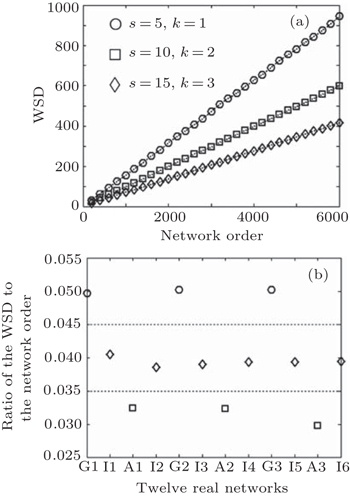
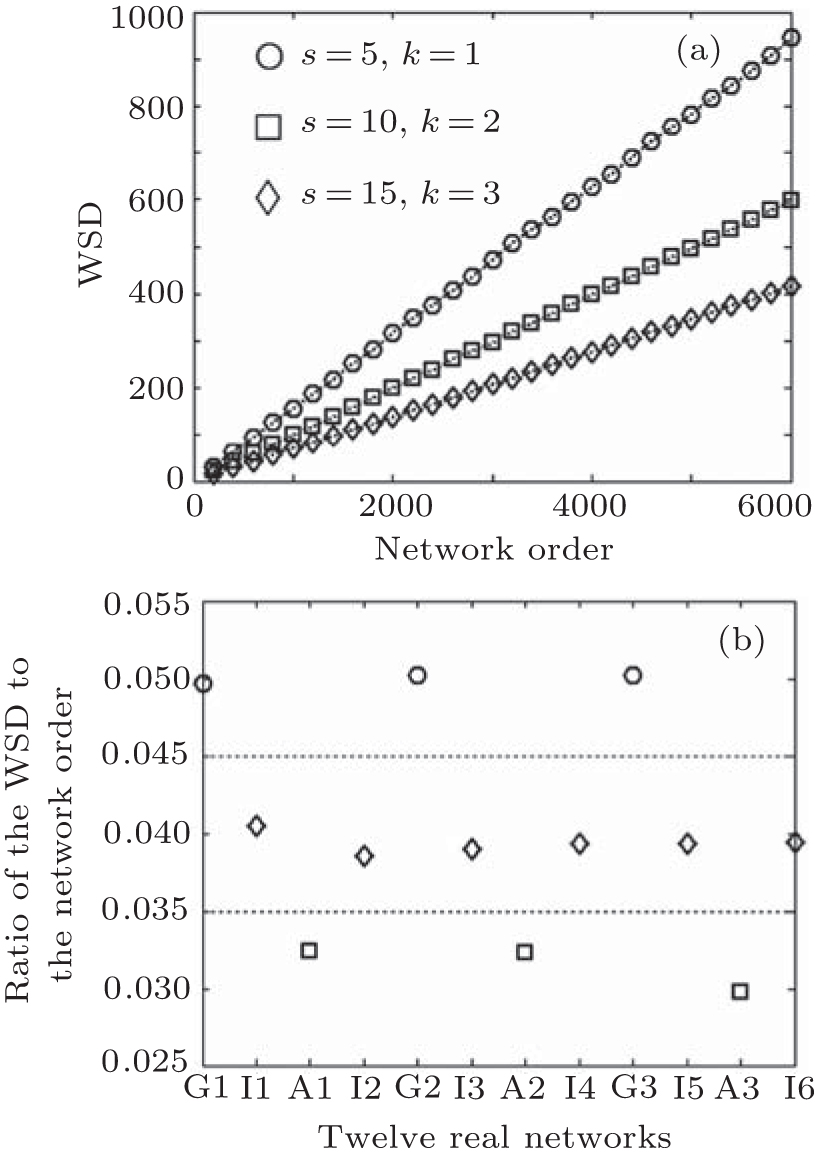
The module generated by Watts–Strogatz model includes s nodes. Specifically, each node in the module is first connected with its 2k neighbors, and then each edge of the node is randomly rewired with a probability α. As shown in Fig. 2(a), when m = 3 and α = 1, by using different inputs s and k, Zou’s model can simulate diverse evolving networks with different modules. Figure 2(a) shows that for a certain module corresponding to unaltered inputs s and k, the WSD grows sublinearly as the network order increases. Additionally, figure 2(a) shows that the ratio of the WSD to the network order is a good indicator which can be used to distinguish evolving systems with different modules.
Furthermore, we choose 12 real-world networks with different orders,[1] as shown in Table 1. Specifically, in Table 1, G1, G2, and G3 correspond to a sequence of snapshots of the Gnutella peer-to-peer file sharing network, I1, I2, …, I6 correspond to a sequence of snapshots of the autonomous-system-level Internet topology, and A1, A2, and A3 are networks that were collected by trawling Amazon website.
Table 1.
Table 1.
 Table 1. Twelve real-world networks with different orders.[1] .
| Item |
Node number |
Edge number |
Snapshot time |
|---|
| G1 |
22687 |
54705 |
Aug 25 2002 |
| I1 |
16301 |
65910 |
Jan 05 2004 |
| A1 |
400727 |
3200440 |
Mar 12 2003 |
| I2 |
17848 |
74344 |
Sep 06 2004 |
| G2 |
36682 |
88328 |
Aug 30 2002 |
| I3 |
19846 |
80970 |
Jul 04 2005 |
| A2 |
410236 |
3356824 |
May 05 2003 |
| I4 |
21901 |
89176 |
May 01 2006 |
| G3 |
62586 |
147892 |
Aug 31 2002 |
| I5 |
24454 |
99660 |
Mar 05 2007 |
| A3 |
403394 |
3387388 |
Jun 01 2003 |
| I6 |
26475 |
106762 |
Nov 05 2007 |
| Table 1. Twelve real-world networks with different orders.[1] . |
As shown in Fig. 2(b), we calculate the ratio of the WSD to the network order in the twelve real-world networks listed in Table 1. Figure 2(b) shows that the ratio indeed is a good indicator which distinguishes evolving systems.
6. ConclusionOur recent work[4,5] numerically verifies that the WSD increases sublinearly in a stochastic evolving scale-free network model as the network order increases. However, the stochastic models using interactive growth mechanisms are not suitable for the rigorous analysis of the scaling feature of the WSD. In this paper, our contributions focus on the derivation of the WSD’s precise formula in a deterministic model which captures the scale-free, small-world, and hierarchical features of many real-world networks. The precise formula rigorously explains the WSD’s stability (i.e., the ratio of the WSD to the network order is bounded as the network order increases). The stability indicates that the WSD can be applied to compare different order networks and to distinguish diverse evolving systems whose network orders grow over time.


 , Nie Yuan-ping2, Huang Cheng-dong1, Du Jing1, Guo Rong-hua1, Huang Fei1, Shi Jian-mai3]