1. IntroductionIn modern density functional computation of electronic structures, the exchange correlation potential is a functional of the electron density.[1] If the latter is known, we can further determine a lot of the ground state properties, such as total energy and its derivatives with respect to other variables such as atom positions, strain or electric field.[2] However, we can only set up an approximate electron density from the start, then calculate the exchange-correlation potential to solve the Kohn–Sham (KS) equation[1] to get single-particle states and build a new electron density through the Fermi–Dirac distribution.[3,4] Mixing the previous and current output electron density to generate a new input electron density and the exchange-correlation potential for the next cycle of solving the Kohn–Sham equation. The iteration continues till a converged electron density and the single-particle energy eigenvalues are obtained. Mixing the electron density properly and solving the Kohn–Sham equation either in matrix eigenvalue form or in differential equation form consist of a self-consistent field (SCF) computation process.
In crystal solids, we may use the space periodicity to expand the electron density and the potential over the discrete reciprocal lattice vectors in the reciprocal space, and use the plane wave basis or other proper basis functions to transform the KS equation into a matrix-eigenvalue form. In this way we can fully adopt the linear algebra methods to get energy bands and wave functions.[3,4] The VASP code has been implemented in the following density mixing schemes:[3,4] linear mixing, Kerker mixing,[5] Broyden mixing,[6] and Pulay mixing.[7] Different reciprocal lattice vector components of density may have different mixing weights.[3] The Broyden mixing algorithm used in the electronic structure computation is adapted from Broyden’s original iteration method[8] and was first proposed by Vanderbilt and Louie[9] and refined by Johnson,[6] Kresse et al.,[3] and Eyert.[10] Among all of electron density mixing algorithms, Broyden electron density mixing (BEDM) has been most often used in the SCF computation in VASP code.[3] This algorithm uses the multiple-step recursive equations to calculate the inverse Jacobian matrix. In contrast, Eyert proposed a very simple BEDM algorithm without recursion.[10]
In this paper we compare two BEDM algorithms through the electronic structure computation of a Si atom under the local density approximation.[3,4] The KS equation is solved by using the conventional outward/inward integration of the differential equation and then connecting two parts of solutions at the classical turning points.[11] It is different from the method of the matrix eigenvalue solution as used in the VASP code. As the BEDM is nonlinear, the resulting electron density needs a rescaling in order to keep the charge conservation. In addition, we find that when the BEDM is used, we must use the shooting method to search the accurate energy eigenvalues for shallow bound states instead of using the energy eigenvalue correction formula, which is expressed through the first-derivative discontinuity of radial wave functions at the connection point and can be found in the textbook.[11] In the shooting method, a lot of guessed energy eigenvalues are chosen and then the outward/inward integrations of the differential equation are performed to see whether two parts of solutions can be connected with the smooth first derivative at the classical turning points. It is a very time-consuming process. In contrast, it is found that in the linear electron density mixing (LEDM) we can use this perturbation correction to calculate the estimation of the energy eigenvalues in the next cycle and obtain the converged results. Our results show that the BEDMs need less iteration numbers but longer computation time compared to the LDM. Of the two BEDM algorithms, to reach the same converged results, the one proposed by Eyert takes less total iteration numbers.
2. Theoretical basis2.1. Relation among the Newton–Raphson method and several Broyden methodsThe BEDMs used in this paper are different from Broyden’s original methods and belong to the so-called modified Broyden methods.[3,6,10] Eyert has given a very good account of relations among the Newton–Raphson method, Broyden iteration methods, and the modified Broyden methods.[10] For readers to better understand the Broyden methods we give a simple explanation here.
A multi-dimensional iteration may be defined as a nonlinear operator which when applied to an input vector ∣x(m)⟩ of length N produces an output vector ∣y(m)⟩ of the same length. Here we have used the Dirac state symbol. The superscript m (m ≥ 1) denotes the iteration number. Although the input and output vectors often take the electron density in the computation of electronic structures, they can be any variables. We define a residual vector as follows:

In the second step we have written |
R(m)⟩ as multi-dimensional functions of the input vector |
x(m)⟩. Self-consistency is achieved when the residual vector vanishes, so |y
(m)⟩ = |
x(m)⟩. In actual iterations, it is the length of the residual vector that is used to measure the convergence. Hence, an inner product is usually defined in the space spanned by input and output vectors. The inner product also induces a norm in the same space. The norm of the residual vector is formally written as ⟨
R(m)|
R(m)⟩.
In the (m + 1)-th iteration, the residual vector can be linearly approximated as

Here
J(m) is the Jacobian matrix, defined by

If the residual vector on the left side of Eq. (
2) is required to vanish, we obtain the following proposal for the new input vector:

If we know the analytical dependence of |
y(m)⟩ on |
x(m)⟩ and the dimension
N is small, we can use Eqs. (
1) and (
4) to obtain a new input vector |
x(m + 1)⟩. At each iteration step, we calculate the exact Jacobian matrix
J(m) at |
x(m)⟩ from Eq. (
1), invert it, and then calculate |
x(m + 1)⟩ by using Eq. (
4); it is the so-called Newton–Raphson method.
In most cases, the exact Jacobian matrix is not available. In the m-th iteration we use an approximated one in Eq. (4) to calculate a new input vector |x(m + 1)⟩ and the corresponding residual vector |R(m + 1)⟩. To continue the iteration, the following difference vectors are defined:


To get an estimate of J(m + 1), we require it to be the following equation:

Far away from the final solution, the residual vector |R(m + 1)⟩ does not vanish. Equation (14) fixes only the projection of the new Jacobian on the vector |Δ x(m)⟩. The update J(m + 1) − J(m) fulfills a similar equation,

To determine J(m + 1) completely, J(m + 1) − J(m) can be formally written as

where
I is the unit operator and the second term presents the projection of the update onto the space orthogonal to |Δ
x(m)⟩. Broyden argued to neglect the second term and obtained the following rank-1 update formula:
[8]

The initial Jacobian matrix
J(1) can be taken as a constant diagonal matrix,

Here
IN×N is the
N ×
N unit matrix and the parameter
β is in the range of 0 <
β < 1. Equations (
1), (
4), (
9), and (
10) form an iteration process. In the above method we update Jacobian
J(m) directly. It is called Broyden’s first method. The drawback of this method is that when
N is very large, we have to store very large
N ×
N matrices and calculate the matrix inverse used in Eq. (
4). Broyden’s second method uses the inverse Jacobian matrix
G(m) = (
J(m))
−1 directly and thus avoids calculating the matrix inverse. Corresponding to Eqs. (
4), (
5), (
9), and (
10), we have


Both Broyden’s first and second methods need to store large N × N matrices and only use the iteration information in the last step. Vanderbilt and Louie proposed to use iteration information in the previous several steps of iteration.[9] For example, if the inverse Jacobian matrix is used to perform iteration, instead of Eq. (12), we require G(m + 1) to fulfill the following M equations:

In this way, we can use all the iteration information in the previous
M steps of iteration. Eyert has shown how to define a projection operator and then followed Broyden’s argument to derive an equation of
G(m+1) based on
G(m+1−M), |Δ
x(l)⟩, and |Δ
R(l)⟩ for
l =
m+1−
M,…,
m. For the initial guess for inverse Jacobian matrix, we use

Such iteration methods are called modified Broyden methods. Johnson and Eyert applied the method to the self-consistent electronic structure computation using the electron density as iteration vectors.[6,10] They reformulated it by using the variational schemes to determine G(m+1) through the definition of cost functions. In the following we give some details.
2.2. Implementation of BEDMs during SCF computationDuring the SCF computation process, given an input electron density ρin, we generate an output electron density ρout through solving the KS equation. The self-consistency respect to ρin requires that the charge density residual vector R[ρin][3]

is zero.
ρout and
R[
ρin] are both complicated functional of
ρin. Let us denote

as the input electron density in the
m-th step of iteration. In the BEDMs, it is assumed to be near the zero value of
R[
ρ],

As no explicit analytical dependence on
ρin is available for
ρout, it is impossible to compute the exact Jacobian matrix, so we have to take an approximation for
J(m). To require
R[
ρ] = 0, we gain an optimal charge density
ρ* in the form of

In successive steps, an improved approximation of inverse Jacobian matrix
G(m) ≡ (
J(m))
−1 is built up based on Broyden’s second method and a new charge density is obtained from the current approximation of inverse Jacobian matrix
G(m), the current charge density

, and the current residual vector

through the following equation:

Here equation (20) clearly shows the forming of  through the density mixing.
In Johnson’s BEDM algorithm, information of all previous steps of iterations is used to calculate G(m) for the current iteration. For the m-th iteration, this is done via a least square minimization of the following error function:

Here we have defined


In the first and second terms of Eq. (
21), the Frobenius matrix norm

and the vector norm

are used, respectively.
[6] For weight factor
w0 and
wi, the relation
w0 <<
wi fulfills.
[3,6] Minimizing the error function in Eq. (
21) with respect to
G(m+1), we can derive a set of recursive equations for
G(m+1) in terms of
G(1), |Δ
ρi ⟩ and |Δ
Ri ⟩ with
i = 1, 2, …,
M,
M + 1. After completing
M + 1 steps of recursive iterations, we reset
G =
G(1) =
β IN×N and restart the next cycle of recursive iterations. Our implementation of this BEDM uses the corrected equations given by Kresse
et al.
[3] The original equations given by Johnson have several mistakes.
[3,6] Eyert proposed to minimize the following error function to get
G(m + 1):
[10]

where
aij = ⟨Δ
Ri| Δ
Rj ⟩ and
G(m+1− M) =
β IN×N.
M is the iteration depth and is the same as in Johnson’s algorithm. Weight factors in Eqs. (
21) and (
23) may be different, but the relation
w0 <<
wi fulfills in both BEDM algorithms.
[3,6] Minimizing the error function in Eq. (
23) with respect to
G(m), we can derive a very easy equation for
G(m) without using recursion. Further we can derive an iteration equation for


The quantities of

are defined in Eyert’s paper and can be easily calculated through solving a small set of linear algebra equations.
[10] However, the definition of the inverse Jacobian matrix here has one minus symbol difference and is the same as that used by Kresse
et al.
[3] Compared to those complex equations for
G(m) in Johnson’s algorithm,
[3,6] Eyert’s algorithm does not even need to calculate and store
G(m).
[10]To better distinguish a BEDM from the other, we further denote Eyert’s BEDM as BEDM1 and Johnson’s BEDM as BEDM2. In the following we explain how to use these BEDMs to compute the atomic electronic structure.
2.3. Solving KS equationAs usual, we use the following transformation to discrete the radial coordinate:[10]

Here,
r0 is a constant. The uniform discretion in
x with a step of
h gives a discretion which is dense in small
r and dilute in large
r. With this variable transformation, differentiation and integration with respect to
r can be changed into those with respect to the variable
x: d
r =
rd
x. We denote the uniform
x-discretion points as
x1,
x2, …,
xN with an increasing order. Correspondingly we have a set of non-uniform
r-points:
r1,
r2, …,
rN. Here,
N is the number of total discretion points.
The spherical averaged radial electron density ρ(r) and the bulk electron density n(r) fulfill the following equations:


Here,
Z is the atomic number of an atom and for Si,
Z = 14.
The KS equation for the ground state in a spherically symmetrical potential is

where
VHXC(
r) is the Hartree potential plus the exchange–correlation potential. The Hartree atomic unit is adopted:
me = 1,
ħ = 1, and
e2 = 1. The wave function can be written as

The normalization is implemented through

. With the introduction of
ϕnl (
r(
x)), the following form is obtained:

Given a guess of the eigenvalue
Enl, this equation is integrated both outward and inward using Numerov’s method.
[11] At the exact eigenvalue
Enl, two pieces of wave function are connected with smooth 0-th and 1-st derivative of

at the classical turning point
rctp. If

is not continuous in two sides of point
rctp, the following improvement to the eigenvalue
Enl in the (
m + 1)-th iteration can be estimated from the
m-th iteration:
[11]

Here,
δ is a very small positive number used to define the left and right derivative of
χnl with respect to
r. In addition to using this correction formula (denoted as E-pert), we also try the shooting method (denoted as shooting) to search for the exact energy eigenvalue based on the discontinuity of

in a certain energy window. Compared to the E-pert method, the shooting method is slower, but has a higher accuracy.
In the LEDM, the (m + 1)-th input density  is calculated by

In this scheme, if both

and

are normalized according to Eq. (
26),

is also normalized.
2.4. Defining the discrete radial electron densityWe now define  vector in a BEDM as

Here,

and the transpose operation ‘′’ has been taken to define

as a column vector.

is a weight matrix. A similar definition applies to

with the same weight vector. One choice is to choose
Swr as an
N ×
N matrix identity matrix,

The other choice of the weight matrix is

Here,
N is further assumed to be an odd integer. Equation (
34) originates from making the variable transformation from
r to
x and then performing a numerical integration with the Simpson rule in the left of Eq. (
26b). Other choices of weight matrix are also possible. With such definitions of column vector

and

, we can compute

,

,

and the corresponding inner products very easily. For example, if equation (
34) is chosen for the weight vector, the following inner product is calculated:

To summarize, in the LEDM we use the density column vector defined by Eq. (31). In BEDMs we compare two definitions (Eqs. (33) and (34)) of the density column vector; the reason to do this is that in solids, especially in metals, proper weight factors are needed to avoid charge sloshing. To analyze convergent properties in different schemes (different density mixing and different weight vector to define the different column vector  for iteratively computing the Jacobian matrix G(m)), the following quantity is used:

Here the same set of weight factors defined in Eq. (
34) are used in all schemes to fairly compare the convergent error defined by

.
3. Results and discussionWe take β = 0.3 in the initial inverse Jacobian matrix and in Eq. (31). We set w0 = 0.01 and wi = 1 in Eqs. (21) and (23). The iteration depth in two BEDM algorithms is taken as M = 5. The hydrogen wave functions are used as the input. For the exchange–correlation potential, we have tested both the local density approximation (LDA)[12] and the generalized gradient approximation using the PBE functional.[13] It is found that the convergence behaviors in both cases are very similar, so we only present the results based on LDA. As in the initial cycles, there appear the drastic variations of VHXC(r), wave functions and the corresponding Enl, the stable algorithms of the shooting method plus the LEDM are used in the first 5 times of iterations. With M = 5, each cycle of BEDM corresponds to 6 times of iterations in the LEDM. So we compare two BEDMs in 100 cycles and the LEDM in 600 times of iterations. It should be emphasized that two kinds of weight matrices (Eqs. (33) and (34)) are used to define the different column vector  for iteratively computing the inverse Jacobian matrix G(m) to see the effect of different choices of weight matrices. In the convergent error
  ,
,  and
and  are converted into forms defined using the same weight vector in Eq. (34).
Figure 1 shows the calculated radial electron density ρ(r) after 600 times of iterations under three conditions: (i) LEDM, E-pert; (ii) BEDM1, E-pert; and (iii) BEDM1, shooting. It can be seen that ρ(r) in cases (i) and (iii) are the same, while in case (ii) the highest peak of ρ(r) is missing. This peak corresponds to 3s and 3p states with small absolute value of Enl. The wave functions of these states are very sensitive to the error of Enl. Figure 2 shows the corresponding convergent errors in three cases. In cases of (i) and (iii), it decreases rapidly with the iteration number, while in case (ii), it retains very large values even after 200 times of iterations. Its final decrease after 250 times of iterations gives completely wrong wave functions for 3s and 3p states in a large r region. The shooting method is more accurate, but it is too slow. To accelerate the iteration speed, we have adopted a compound method: for core states the E-pert method is used to get new values of Enl, for valence states such as 3s and 3p states, the shooting method is used with a much smaller energy search window. It greatly enhances the computation speed. The results are calculated using this method. The trends in Figs. 1 and 2 do not depend on the BEDM and weight matrix.
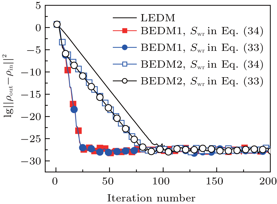
Figure 3 shows the convergent error in LEDM, BEDM1, and BEDM2. It is found that two kinds of weight matrices used to calculate  and G(m) hardly affect the convergent error. With respect to the iteration time, BEDM1 is the fastest, LEDM is the slowest and BEDM2 is in between. The conservation of charges in the BEDM iteration process is also examined. With the atomic number Z = 14 and the input total electron number of
  before renormalizing ρin(r) to Z, in all four iteration processes with the BEDM shown in Fig. 3, the quantity (Ne − Z)/Z decreases from −1.9 × 10⁻¹¹ to −2.3 × 10⁻¹¹ after 1 cycle of the BEDM iteration and stays almost constant during later iterations. This means although the BEDMs are nonlinear, the charge conservation almost keeps with present choices of weight factors.
Figure 4 compares the converged radial electron density ρ(r) and those after 1 cycle (6 times of iterations) of BEDM1 and BEDM2 iteration process. The profile from BEDM1 is in much better agreement with the converged result. As both start from the same initial electron density and the same initial Jacobian matrix, this result indicates that BEDM1 is more accurate than BEDM2.
Finally using Eq. (24) we easily show how the weight matrix affects the iteration vectors. We can easily prove the following equation:

The same transformation matrix

applies to the transformation of |Δ
ρ(m)⟩, |
R(m)⟩, and |Δ
R(m)⟩. In this way we can transform the iteration vectors from weight matrix
Swr1 to
Swr2 very easily. Meanwhile neither the initial inverse Jacobian matrix nor the form of Eq. (
24) will change.


 ]
]