The motions of interacting entities have drawn attention in various fields.^[1,2] They contain ants, birds, pedestrians,^[3,4] vehicles, and even robots, which are termed as self-driven particles.^[5–8] Many phenomena in these systems have been studied, such as phase transitions and metastable states.^[9–11]

Chasing, which is ubiquitous in nature, has been investigated for a long time. A two-particle system consisting of one chaser and one target is the simplest case, where there exists a challenging mathematical problem to depict trajectories.^[12–14] Systems with many chasers and one target have been modeled and analyzed.^[15,16] Systems including several chasers and targets have been studied in fields of game theory and multi-agent problems.^[17,18] The chasing problem has been further extended to group chase, considering a lot of chasers and targets.^[19] In this model, each chaser tries to pursue the nearest target, and at the same time each target does their best to escape the nearest chaser in order to avoid removal. In addition, conversion has been added in the model, meaning that the caught targets convert into chasers instead of removals.^[20] Furthermore, some fast chasers have been considered to investigate the optimal number of chasers and minimum cost for catching targets.^[21] Almost all studies on chasing aim at selecting targets dynamically in the process, but ignore the situation in which each chaser has only one constant target, i.e., the regular queue. In many cases, such as marching, members in a queue will always regard the closest one ahead them as targets, and follow the trajectories they leave.

A self-driven particle system covers a wide range, for example the fleet of carrier robots in a future factory. Some unreasonable setting in a queue may lead to chaos. In this work, we study the effect of initial distance and relaxation time on the stability of a queue chase by using a delayed model. In this model each chaser regards the preceding one as a target. We find that when the target of the first member in the queue shows a slight fluctuation, a big fluctuation in the system can generate and neighbors’ distance will change. Increasing initial distance or decreasing relaxation time can enhance system stability, which may be helpful for engineering design. By convergence analysis, the critical parameter values are found.

This paper is composed as follows. The delayed model and parameters are introduced in Section 2. Then we present the simulation results and convergence analysis in Sections 3 and 4, respectively. Section 5 shows the conclusion.

The delayed chasing model selected from Helbing^[22,23] is continuous both in time and space, and we apply it to depict queue chase behaviors. Each chaser regards a particular one (unchanged in the walking process), who locates in the nearest place ahead in the initial stationary state, as the target. According to the sequencing, we set L₁(t) = (x₁(t), y₁(t)) as the leader’s position of the queue, L_n(t) = (x_n(t), y_n(t)) as the location of the final one at time t, and suppose that the queue includes n members. In addition, L₀ denotes the position of the leader’s target.

The chasing force, which represents one’s motivation to walk in a given direction with a desired speed, is influenced by Newtonian-like mechanics and then given by

This relationship reflects the adaptation of current speed v_i (t) of chaser i to a desired speed and a desired direction of motion within a certain relaxation time τ, which means the delay to adjust velocity. From Ref. [24], the relaxation time τ was set as 0.54 ± 0.05 s, and the pedestrian’s common desired velocity is 1.29 ± 0.19 m/s. However, here for a general study, we assume that and τ are variable parameters. In addition, .

Then the resulting motion differential equation reads

Using the delayed model, we have carried out simulations for queues. Firstly, the leader’s target point is distributed in L_o = (x_o(t), y_o(t)), where x_o fluctuates according to the uniform probability distribution in an interval [−f, f] at each time step and y_o(t) is constant 40000 m in all simulations. Before a progress starts to run, the leader occupies the frontal position L₁(0) = (0, 0) in the queue, and all other x_i = 0, dis = y_{i − 1} − y_i, where dis denotes the initial distance between any two neighbors. Figure 1(a) shows the original state at t = 0 s. Because of such a small value of dis, all members form a line-like pattern. Following rules in the model, all chasers update orderly to pursuit their targets. Firstly, the relaxation time and desired velocity are set as 0.5 s and 1.3 m/s. Other parameters for the simulation are Δt = 0.02 s and n = 300.

Fig. 1.

	Figure Option ViewDownloadNew Window
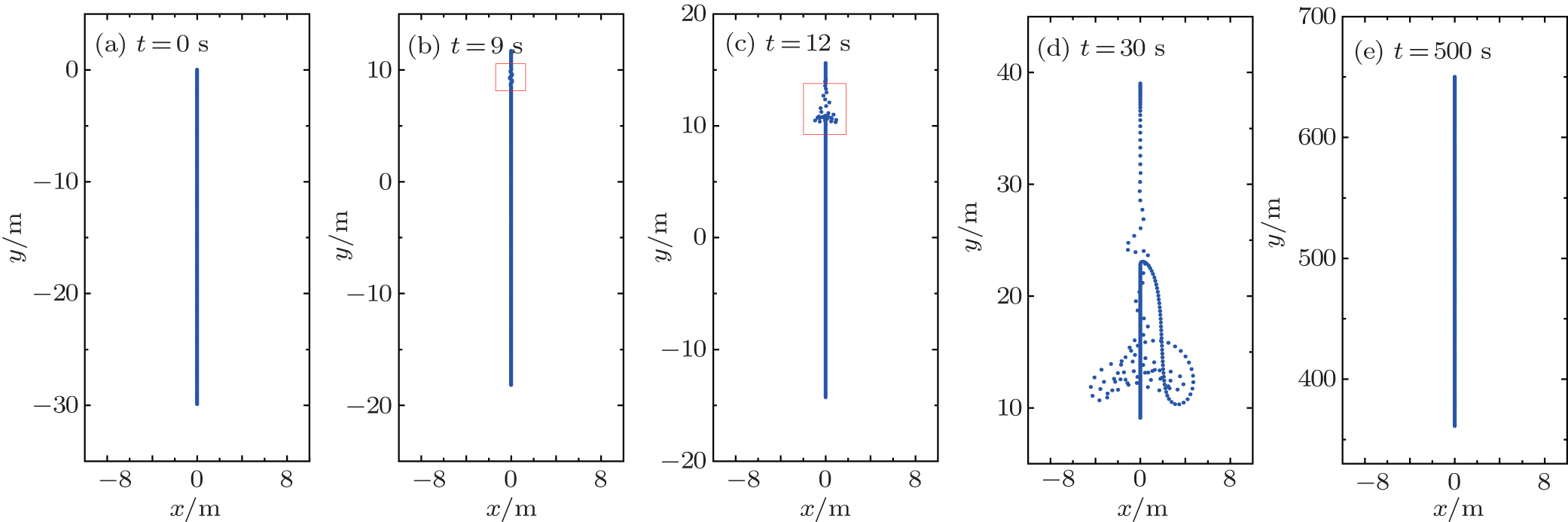	Fig. 1. Changing queue pattern for t = 0 s (a), t = 9 s (b), t = 12 s (c), t = 30 s (d), and t = 500 s (e) when dis = 0.1 m, f = 0.1 m, vo = 1.3 m/s, and τ = 0.5 s.

When f = 0.1 m, all chasers move forward as a line over timescale t ∈ [0 s, 9 s]. At t = 9 s, a series of fluctuations emerge in the red outline of Fig. 1(b). The amplitude of the wave is intensified further over time as described in Figs. 1(c) and 1(d). For the reason that we ignore repulsive forces in our model, figure 1(d) shows horizontal moving chasers move across vertical ones without any response behavior. While the pattern may slightly deviate from the realistic state, this phenomenon reflects one micro disturbance from the origin can bring about qualitative change in its relevant system. After a long time like t = 500 s in Fig. 1(e), all chasers overcome fluctuations in the queue and recover the stabilized line-walk. However, these line-like patterns in Figs. 1(a) and 1(e) have significant distinction in queue length, which are respectively 29.9 m and 290 m. From Fig. 1, we find that if the lateral intertwined phenomenon will not hinder the pursuit course, a queue with finite members could adjust by itself to a stable state, even taking no account of repulsive impacts.

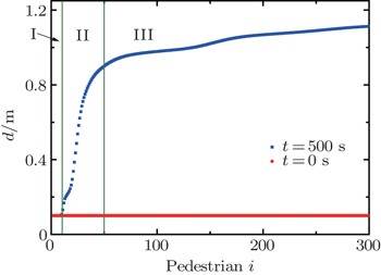
The increment in queue length implies variation of distances between neighbors, which is rendered in Fig. 2. The blue line at t = 500 s can be divided into 3 parts: only the top-ten chasers keep distances with the one ahead in about 0.1 m at region I; then distances enhance sharply from the 11th to approximately 50th pedestrian, arriving at 0.9 m inside region II; at region III, distances of following pedestrians increase slightly to the asymptotic line y = 1.2. It is plausible that there are smaller distances between neighbors in the pursuing (vertical) direction, the bigger offset in the desired direction can lead to the same fluctuation in the horizontal. In other words, a bigger fluctuation means a larger horizontal velocity, and combining the fact that scalar of desired velocity is constant 1.3 m/s, lower vertical speed belongs to the member. As the leader’s vertical speed is basically 1.3 m/s, but some followers, especially like the chasers inside the red outline of Fig. 1(c) and a part in Fig. 1(d), even move along the horizontal direction, the vertical-walking distance between the leader and the last one is significantly distinctive at t = 500 s. Hence, chasers may forgo getting too close to the one ahead to achieve a stable state.

Fig. 2.

	Figure Option ViewDownloadNew Window
	Fig. 2. Distance (d) between neighbors at time t = 0 and t = 500 s. n = 300, dis = 0.1 m, f = 0.1 m, vo = 1.3 m/s, and τ = 0.5 m.

Figure 3 shows disturbance at different values of initial neighbors’ distance dis. In order to quantify the disturbance of the moving queue, an order parameter is introduced as

A larger value of disturbance rate D indicates smaller disturbance. All members move along the same direction if D = 1. For universality, one can define the deviation degree between the direction of the leader’s desired velocity and the vertical as

Numerical simulations reveal that the factor of initial distance dis has significant effects on quantity of disturbance rate and the time, when the lowest D emerges. After different periods of time respective to different dis, disturbances appear. Then before the queue returns to a stable state (D = 1) again, we have collected dissimilar lowest quantity of D (symbolized by D_l), as shown in Fig. 3(a), where the black line reflects the process in Fig. 1.

The effect of variable deviation degree is presented in Figs. 3(b) and 3(c). Figure 3(b) illustrates in detail that with the increasing neighbors’ distance dis, the quantity of D_l in each line is continually enhanced until reaching the upper bound. Besides, the critical point dis_c when D_l arrives at 1, is also higher, as the leader’s target has bigger fluctuating amplitude, namely, f f gets bigger. From Fig. 3(b), one can see that no matter how small the deviation degree f f is, as long as dis is small enough, the deviation rate D can drop to a small value, which means the disturbance generated by the leader’s target point cannot get convergence until there exists a large distance between neighbors. We will discuss the problem of convergence concretely in the next section. Figure 3(c) describes that the quantity of t_l varies at different dis and f f when the lowest D is obtained.

Fig. 3.

Figure Option ViewDownloadNew Window

Fig. 3. (a) Relationship between initial distance dis and disturbance rate D in the time period [0,300 s] with the condition f = 0.1 m. Dl and tl here mean the lowest quantity of D and the time achieving that in the process. (b) Distribution of Dl with variable f f. disc shows that when initial distance dis > disc with one certain f f, D keeps at 1 all the time, i.e., no observable disturbance exists in the queue. (c) Distribution of time tl when relative Dl is obtained.

Fig. 4.

Figure Option ViewDownloadNew Window

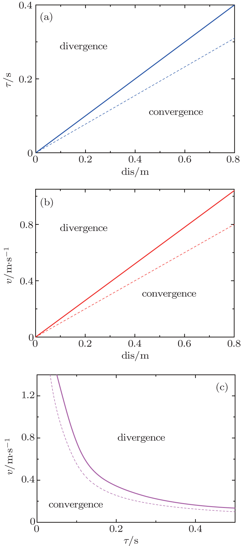Fig. 4. Divergent or convergent transformation process under three variables. (a) Initial distance dis and relaxation time τ with vo = 1.3 m/s. (b) Initial distance dis and desired velocity vo with τ = 0.5 s. (c) Relaxation time τ and desired velocity vo with dis = 0.1 m. Because the value of f f has no qualitative influence on the convergence, f f is fixed at 10−3. The dotted lines are boundaries from convergence analysis.

Figure 4 presents that the initial distance, target velocity, and relaxation time decide whether the queue undergoes the divergence phase. If D_l ≈ 1, which means disturbance does not emerge, these two distances are equal; otherwise the final distance is larger. Since there exists the fluctuation of leader target, the critical value of D_l should be a little smaller than 1. D_l is set as 0.999. If D_l < 0.999, we consider there is a transformation of divergence in the simulation. Otherwise the queue formation is stable, which means the disturbance is convergent. In Fig. 4(a), with the increasing dis, individuals in the queue have more reaction time before resulting in the divergence condition. The relaxation time is linearly related to the initial distance. Figure 4(b) illustrates the similar linear relationship between initial distance and desired velocity as Fig. 4(a). When the initial distance is fixed as shown in Fig. 4(c), with the enhancement of relaxation time, the maximum velocity, which keeps the queue stable, is constantly decreasing. The relationship measures up a hyperbolic curve.

Here, we present the complex function to find which factors have an effect on fluctuation convergence. Figure 5 shows how the first 3 members move in the horizontal direction over time [0, 4 s]. It is plausible that the leader walks along the horizontal direction abiding by general sinusoidal-like distribution with low frequency, and other chasers have greater amplitudes as described in dark gray outlines of Fig. 5. Additionally, the moments display a time-lapse phenomenon when wave crests of the three lines appear.

Fig. 5.

	Figure Option ViewDownloadNew Window
	Fig. 5. First three members’ location change in the direction of x axis. In this simulation, dis = 0.1 m, f = 0.1 m, vo = 1.3 m/s, and τ = 0.5 s. Arrows in magenta outlines show increasing quantity of amplitude and time-lapse effect from the leader to third member.

According to lines in Fig. 5, we assume that the offset in the x direction is

Equations (1) and (2) in the x direction read

Then we set one parameter

Because in the beginning steps

Next, equation (9) is substituted into Eq. (6),

By substituting Eq. (5) into Eq. (10), we have

If all , x_n is convergent with no doubt, because the constraint condition means the upper limit of convergence. Hence,

In the condition of low frequency ω, namely, ω → 0,

In other words, when dis ≥ 2τv^o, the disturbance is convergent and the queue keeps a stable state. Equation (14) reflects similar laws to Fig. 4: the curve to distinguish divergence or convergence with variable initial distance and relaxation time is a linear relationship; desired velocity is also linearly related to the initial distance; relaxation time and desired velocity present a hyperbolic relationship. While the coefficient in Eq. (14) is 2, the simulated value from Fig. 4 is about 3. In the real situation, ω cannot be 0, so the coefficient, as well as critical b and dis corresponding to convergence, should be a little smaller, as presented in Fig. 6. Nevertheless, the final distance of the stable queue after transformation (dis < 1) is larger than the stable phase threshold dis = 1. This phenomenon cannot be explained completely, so we will try to find the reason in the following study.

Fig. 6.

	Figure Option ViewDownloadNew Window
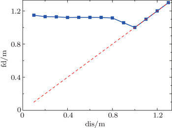
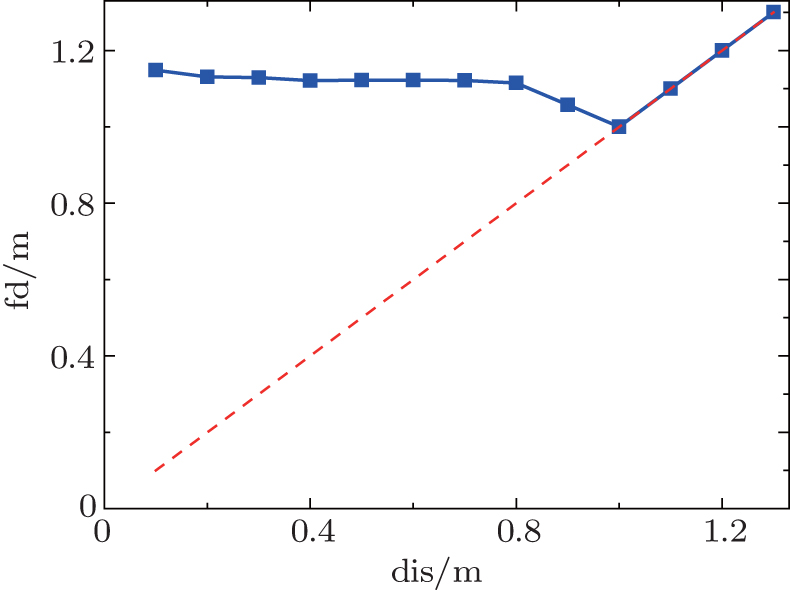	Fig. 6. Distribution of the last two chasers’ (n−1 and n) final distance (fd) with variable dis. The red dashed line means the imaginary final distance in the assumption that disturbance is not divergent. In this simulation, n = 500, f f = 10−5, vo = 1.3, τ = 0.5 s, and time period is [0, 1000 s].

We use a delayed chasing model to mimic chasers in the queue with a slightly fluctuating target of the leader. It is found whether the queue can keep stable state or not depends on initial distance, desired velocity, and relaxation time. At a constant desired velocity and relaxation time, with increasing initial distance, the fluctuation in queue transforms from divergence to convergence. Even if there exists serious disturbance in queue, it will vanish in the end and return to stable with larger distances between neighbors. Moreover, the convergence analysis for this model is carried out, and shows that analytical convergence condition is in approximate agreement with those of simulations. Our results enhance the understanding of queue behavior that chasers should not follow leaders too close or react too slow. This rule may also be utilized in engineering design.