


New data assimilation system DNDAS for high-dimensional models
[Huang Qun-bo1, 2, 3, †,  , Cao Xiao-qun1, 3, Zhu Meng-bin1, 3, Zhang Wei-min1, 3, Liu Bai-nian1, 3]
, Cao Xiao-qun1, 3, Zhu Meng-bin1, 3, Zhang Wei-min1, 3, Liu Bai-nian1, 3]
|
|


† Corresponding author. E-mail:
Project supported by the National Natural Science Foundation of China (Grant Nos. 41475094 and 41375113).
The tangent linear (TL) models and adjoint (AD) models have brought great difficulties for the development of variational data assimilation system. It might be impossible to develop them perfectly without great efforts, either by hand, or by automatic differentiation tools. In order to break these limitations, a new data assimilation system, dual-number data assimilation system (DNDAS), is designed based on the dual-number automatic differentiation principles. We investigate the performance of DNDAS with two different optimization schemes and subsequently give a discussion on whether DNDAS is appropriate for high-dimensional forecast models. The new data assimilation system can avoid the complicated reverse integration of the adjoint model, and it only needs the forward integration in the dual-number space to obtain the cost function and its gradient vector concurrently. To verify the correctness and effectiveness of DNDAS, we implemented DNDAS on a simple ordinary differential model and the Lorenz-63 model with different optimization methods. We then concentrate on the adaptability of DNDAS to the Lorenz-96 model with high-dimensional state variables. The results indicate that whether the system is simple or nonlinear, DNDAS can accurately reconstruct the initial condition for the forecast model and has a strong anti-noise characteristic. Given adequate computing resource, the quasi-Newton optimization method performs better than the conjugate gradient method in DNDAS.
Clifford proposed the dual-number theory in 1873,[1] Yang et al.[2] and Denavit[3] extended the theory. Currently, the dual-number theory is mainly applied in the spatial mechanisms, robot design, matrix mechanics, and spacecraft pilot. Li[4] pointed out the importance of the theory in the spatial mechanisms and robot design. Zhang[5] described the displacement relationship in the spatial mechanisms using the dual-number conception. Wang et al.[6] estimated the rotational motion and the translational motion of the chaser spacecraft relative to the target spacecraft based on the dual-number. Hrdina et al.[7] showed that the dual-number is a proper tool for directly classifying the geometric errors and integrating the multiaxis machines’ error models. The dual-number method is similar to the complex-step approximation; Cao et al.[8] applied the complex-variable method to the data assimilation problems of general nonlinear dynamical systems, and also verified the availability for non-differentiable forecast models. However, the complex-step approximation can only be valid for one variable once, which would lead to very expensive cost for large-scale calculation problems. Yu et al.[9] implemented a general-purpose tool to automatically differentiate the forward model using the arithmetic of dual-numbers, which is more accurate and efficient than the popular complex-step approximation, and the computed derivatives are the same as the analytical results up to machine precision. Andrews[10] utilized dual-number automatic differentiation to analyze the local sensitivities of three physical models. The dual-number may serve as a means to simplify a model or focus future model developments and associated experiments. Fike[11] developed the mathematical properties of hyper-dual numbers and then applied the hyper-dual numbers to a multi-objective optimization method. On this basis, Tanaka et al.[12] proposed a method referred to as hyper-dual step derivative (HDSD), which is based on the numerical calculation of strain energy derivatives using hyper-dual numbers, does not suffer from either roundoff errors or truncation errors, and is thereby a highly accurate method with high stability. Recently, Cao et al.[13] formally introduced the dual-number theory into the community of data assimilation in numerical weather prediction (NWP), and proposed a new data assimilation method.
Variational principles for various differential equations have been investigated for centuries.[14] Currently, the most popular data assimilation methods are 3/4D-Var[15–22] and Kalman filter.[23–25] The aim of data assimilation is to provide accurate initial state information to the discrete partial differential equations controlling the motions of atmosphere or ocean. A data assimilation system optimizes the combination of the observation data and the prior information, and hence provides an optimum estimation of the initial atmospheric state to the NWP model.[26] Taking the incremental 4D-Var as an example, it measures the distances between the analysis states and observations and also the background states. The cost function can be minimized in terms of increments by an optimization algorithm if the first-order derivatives or gradient of the cost function are calculated and provided.[27] Due to the high non-linearity of the atmospheric models and observation operators in NWP, the tangent linear and adjoint techniques are widely applied in the field of data assimilation. The TL model is the first-order linearized approximation of the forecast model with respect to the background trajectory, which is used for computing the incremental updates with perturbations to the initial state variables. The TL model approximately calculates the perturbed model trajectory, then the cost function can be attained.[28] The gradient of the cost function with respect to the initial condition variable is computed by a backward integration of the AD model. Our ultimate goal is to find out the optimal initial condition by an optimization algorithm, of which the gradient of the cost function is very necessary and important input information.
Constructing the TL and the AD models manually is quite complicated and time-consuming, we should first write out the TL model corresponding to the forward forecast model, then construct the AD model. In order to reduce the difficulty of development, the whole forecast model is usually divided into many small segments, and then we write out the TL and the AD models of each segment line by line. Although using this approach makes the development process much simpler, it is still very easy to make mistakes. Furthermore, the actual atmospheric motion equations are very complicated and need some smoothing processes, such as temporal, spatial, and boundary smoothing. These processes will bring great difficulties to us in developing the AD model codes, and sometimes the constructed AD model cannot be completely reversible for the forward integration model.
Because of the drawbacks described above, now a lot of automatic differentiation tools have been developed, such as TAMC[29] and TAPENADE.[30] Automatic differentiation is possibly implemented by the strict rules of tangent linear and adjoint coding. But there are still some unresolved issues. (i) It is still not a black box tool. (ii) It cannot handle non-differentiable instructions. (iii) It is necessary to create huge arrays to store the trajectory. (iv) The codes often need to be cleaned-up and optimized.[27] (v) It has a worse behavior to second- or higher-order derivatives. At present, generating the AD model is not yet fully automatic in reverse mode.[31] It seems that in the foreseeable future, human intervention will be required to finish the most work of AD in reverse mode.[32]
The optimization algorithms play a very important role in the variational data assimilation systems. There are two series of classical optimizing algorithms: gradient-type method and Newton-type method.[33] The gradient-type method (such as conjugate gradient method, CG) requires only the first-order derivative information, which can be directly employed to large-scale unconstrained optimization problems. But for a non-quadratic cost function, the performance of the CG method deteriorates sharply accompanied by a slow convergence speed. The Newton-type method minimizes the cost function by using the information of the second-order Hessian matrix, and the convergence speed is generally faster than the gradient-type method. In practice, the Hessian of most cost functions are not positive definite symmetric matrices which cannot be represented by an analytical solution, leading to using only the first-order derivative of the cost function (which is called as quasi-Newton method). So far, the BFGS is generally thought to be the best quasi-Newton method which can keep the algorithmic global convergence even if it only uses the one-dimensional inexact searching.
At each iteration of the optimization calculation, it inevitably involves solving and saving the first-order and the second-order Hessian matrix information of the cost function. Furthermore, the dimension of the atmospheric state variables can be up to 108–109 in the data assimilation system. Generally, high-dimensional models have the natural attribute of high nonlinearity, and the majority of the geoscientific systems exhibit strongly non-linear characteristics which are also known as “the curse of dimensionality”.[34] Currently, the linearization numerical approximation schemes are frequently-used in NWP for high-dimensional data assimilation, these approaches would give rise to high resolution regional forecast departure occurring owing to the convergence problems and the calculation accuracy problems. There is a corresponding relationship between the adjoint space and the dual-number space derived from the original space in mathematics. They are equivalent to the adjoint state vector and the model state vector. The dual-number operational rules applied in this paper are strictly without any assumptions and approximations, the convergence and precision of the dual-number method can meet the computing requirements of high-dimensional models. How to quickly and accurately calculate the cost function and its gradient information by optimization algorithms is an important question. Nonlinear differential equations generally do not have analytical solutions, which could be replaced by numerical approximate solutions. However, certain characteristics of the equations tend to be ignored because of the machine truncation error.[35] The most attractive feature of DNDAS is that it can efficiently and accurately calculate the first-order derivative information without TL and AD models.
In this paper, we design an attractive new data assimilation system, dual-number data assimilation system (DNDAS), based on the dual-number automatic differentiation principles. DNDAS can accurately determine the cost function and its gradient without developing TL and AD models. The structure of this paper is organized as follows. The following section introduces the dual-number automatic differentiation theory. Section 3 presents the designed architecture of the DNDAS. Section 4 discusses two optimization algorithms. Section 5 analyzes the results of the simulated data assimilation experiments. Finally, conclusions and plans for future work are given in Section 6.
A dual-number x̂ can be expressed as a pair of ordered real numbers x and x′

The dual-number function is expanded into Taylor series


To obtain the derivation of arbitrary function f (
In order to compute cost function J(
In variational data assimilation, the cost function is usually defined as
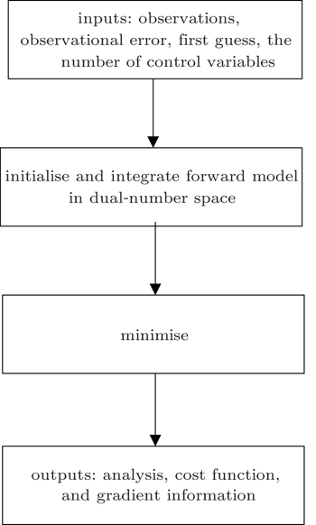
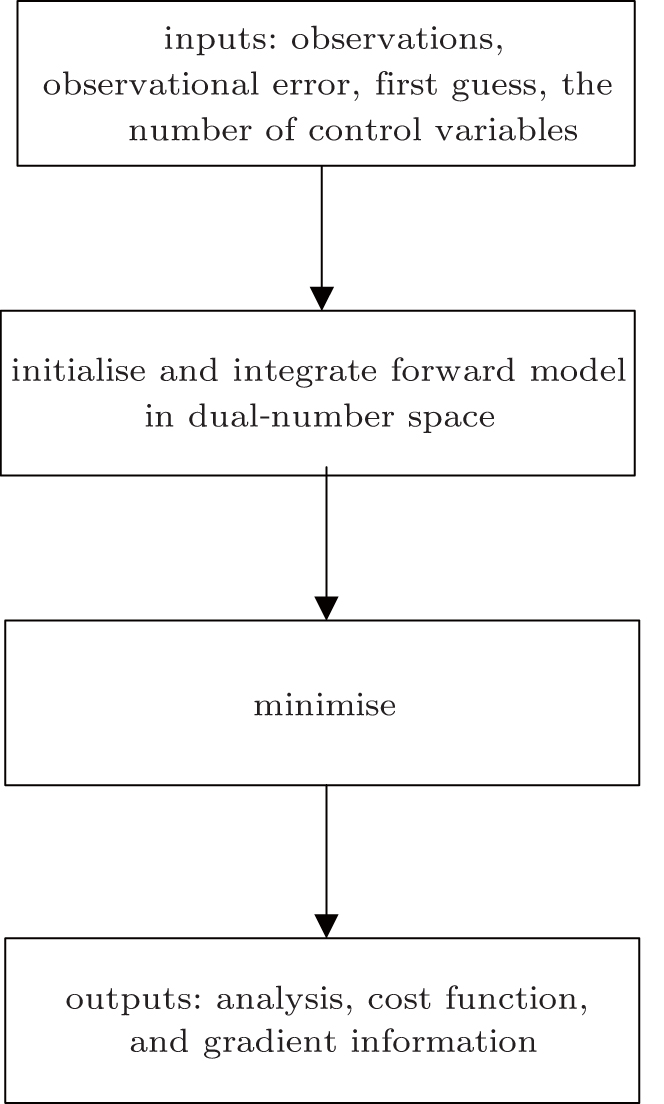 | Fig. 1. Frame of DNADS. |
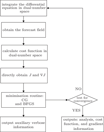
 | Fig. 2. Minimise and output. |
Note that, the convergence criterion ∥∇
After obtaining the cost function and its gradient vector, a descent algorithm is chosen to determine the optimal initial state of the forecast model. Optimization or minimization problems have the general form: min f (
In this paper, the conjugate gradient algorithm is the Beale restarted memoryless variable metric algorithm.[36] The quasi-Newton algorithm is the BFGS variable metric method.[37] For convenience, the conjugate gradient method is called CG, the BFGS variable metric method is called BFGS. CG and BFGS both use the Davidon cubic interpolation[38] as the basic linear search method to find the best step length. During the calculation process, the step length α must obey the Wolfe criteria,[39] which are


The steepest descent direction selected by CG has the feature of conjugacy, so only the first-order derivative information is required during the calculation. The algorithm is described as follows.[40]


The BFGS method requires the cost function to be convex and twice continuously differentiable. The iterative solution can be written as[41]


The calculation process of BFGS is similar to that of CG, but there are some differences between them. BFGS considers the impact of the scale factor and updates matrix
Carbon-11 is a radioactive element with a decay rate of 3.46%/min. The attenuation constant is λ = 2.076 s−1. The atomic number density is A0 at t = 0. The atomic number density differential equation is

This first-order ordinary differential equation is treated as a simple dynamic system. Our goal is to assimilate the accurate initial state of the atomic density by using DNDAS.
In the experiment, we integrate Eq. (
The first guess of the atomic density is set as Ab = 8.5. Considering that the observation should be sparse in reality, three observations at 2nd, 4th, and 6th time steps are selected.
Without considering the background information in the experiment (merely considering the observation influence), the discrete form of the cost function is

The dual-number variable corresponding to the initial background variable Ab is Â0, Â0 = Ab + ε. Then, we perform forward integration in the dual-number space to obtain Ĵ(Â), whose real unit is the original cost function J and dual unit is the gradient
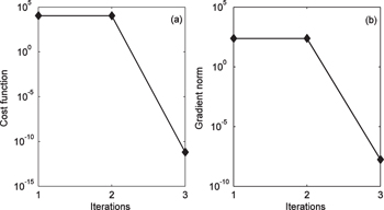
Figures
 | Fig. 3. Trends of (a) the cost function and (b) its gradient norm. |
Figure
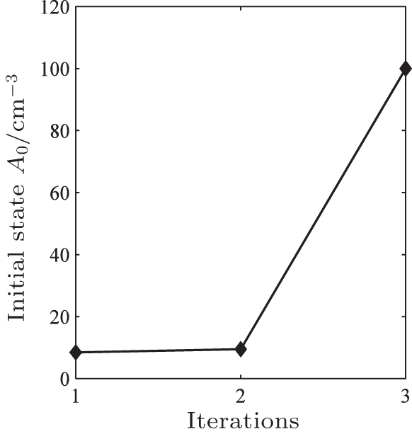 | Fig. 4. Trend of initial atomic density A0. |
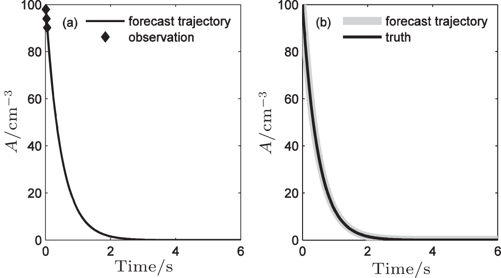 | Fig. 5. (a) Comparison between the assimilated forecast trajectory and observations, and (b) comparison between the assimilated forecast trajectory and the true trajectory. |
However, there are always errors in the observation data, including observation operator errors and so on. Therefore, we consider the validity of DNDAS with Gaussian observational errors δ = 0.1 and δ = 0.2 in the observational sequences, respectively. Table
| Table 1. The assimilation results at different observational error levels. . |
Lorenz-63 chaotic system is the most famous nonlinear dynamic system, which is the first example of chaotic dissipative system.[43] The basis of optimal control to the chaotic system is to control the highly sensitive initial state.[44] Therefore, how to obtain the accurate initial conditions is crucial. The Lorenz-63 model equations are


We integrate the Lorenz-63 equations forward by the fourth-order Runge–Kutta method in the real number space, with the true initial condition of the model
Set the first guess of the model as
The cost function is defined as follows (without considering the background information):

The dual-number vector corresponding to the initial background vector 
The calculation process of the Lorenz-63 model is similar to that discussed in Subsection 5.1, and we will investigate the impact of two different optimization methods on the DNDAS.
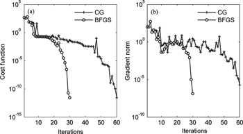
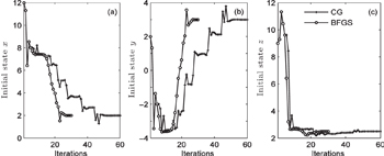
For the cost function and its gradient, without observation error (δ = 0), CG and BFGS can quickly reach convergence after 60 iterations and 30 iterations, respectively, and obtain the same accuracy (Fig.
 | Fig. 6. Trends of (a) the cost function and (b) its gradient norm. |
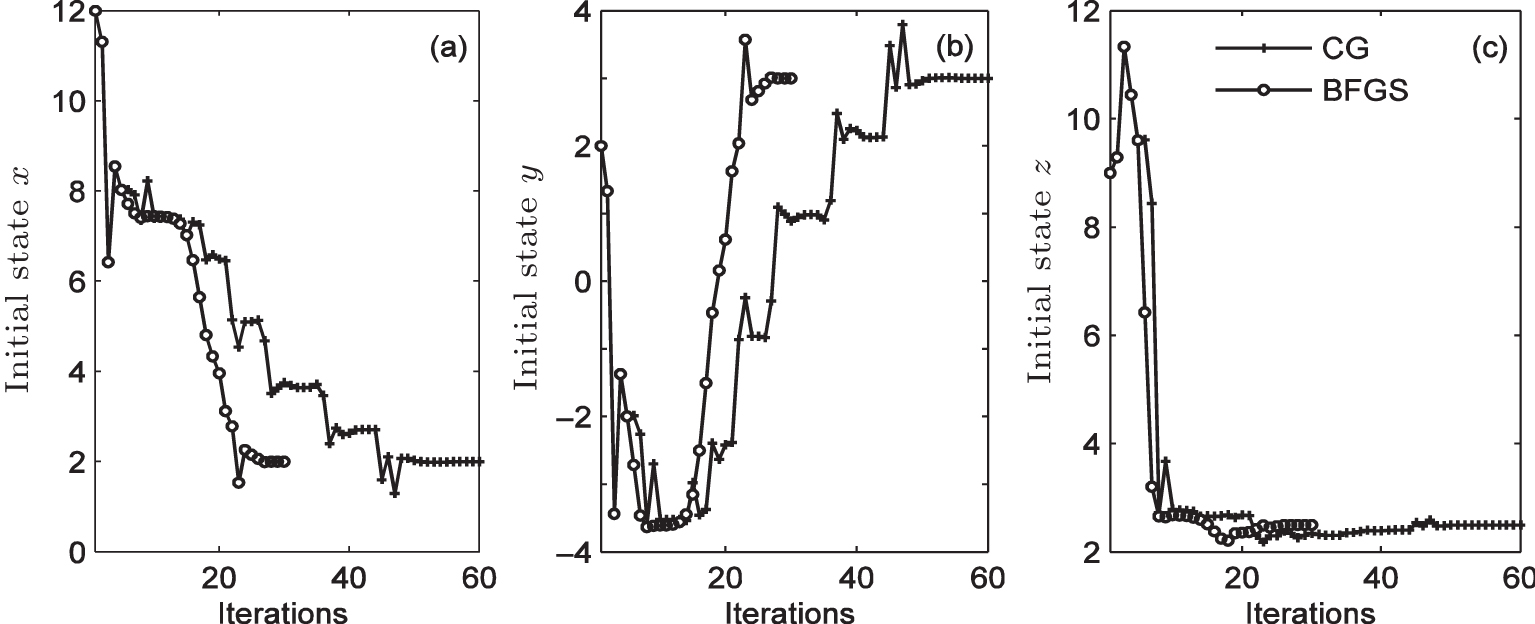 | Fig. 7. Trends of variables (a) x, (b) y, and z. |
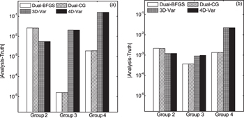
To verify the validity of the DNDAS under the existence of observation error, we have done four groups of experiments (experiment groups 1–4) with δ = 0.0, δ = 0.1, δ = 0.2, and δ = 0.5. In each group of experiment, we evaluate and compare the performances of DNDAS (with BFGS and CG methods), 3D-Var, and 4D-Var, wherein 3D-Var and 4D-Var utilize the identical observation conditions and background conditions as used by DNDAS. Table
| Table 2. Assimilation results at different observation error levels. . |
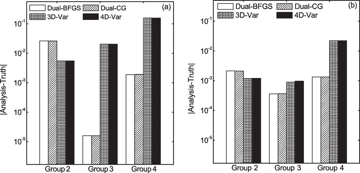 | Fig. 8. The absolute values of departures (analysis minus truth) of variables (a) y and (b) z in the experiments. |
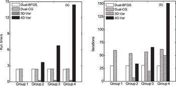
Finally, it is found that, for small-scale problems, the running times of CG and BFGS are nearly the same (see Fig.
 | Fig. 9. (a) Running time and (b) iterations in the experiments. |
The Lorenz-96 model is a dynamical system which was introduced by Lorenz in 1996.[45] The model equations contain quadratic, linear, and constant terms representing advection, dissipation, and external forcing. Numerical integration indicates that small errors (differences between solutions) tend to double in about 2 days.[46] It is defined as follows:

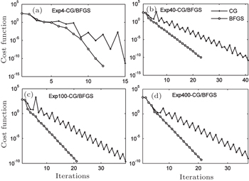
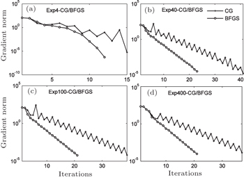
We conduct four groups of experiments, the numbers of control variables are 4, 40, 100, and 400 respectively, and two optimization algorithms (CG and BFGS) are both applied in each group; these experiments are named Exp4-CG/BFGS, Exp40-CG/BFGS, Exp100-CG/BFGS, and Exp400-CG/BFGS.
We integrate the Lorenz-96 equations forward 1000 steps with time step length Δt = 0.001 by the fourth-order Runge–Kutta method in the real number space. The true initial condition of the Lorenz-96 model is
The previous 100 integral values are divided into 10 intervals in order. The observations are obtained by taking the last value in each interval. Due to the high precision of the fourth-order Runge–Kutta method, we take observations as unbiased.
The first guess of the forecast model is
The cost function is defined as follows (without considering the background information):
Subsequently, we construct the dual-number vector as

The whole calculation process is similar to that described for the Lorenz-63 experiment. Next we provide the results of our assimilation experiments.
Figures
 | Fig. 10. Trends of the cost function: (a) Exp4-CG/BFGS, (b) Exp40-CG/BFGS, (c) Exp100-CG/BFGS, and (d) Exp400-CG/BFGS. |
 | Fig. 11. Trends of the gradient norm: (a) Exp4-CG/BFGS, (b) Exp40-CG/BFGS, (c) Exp100-CG/BFGS, and (d) Exp400-CG/BFGS. |
Figure
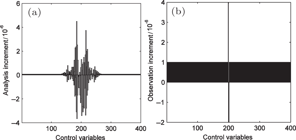 | Fig. 12. (a) Analysis increment and (b) observation increment of each control variable in Exp400-BF experiment. |
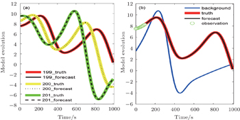
In addition, we restart the forecast model with the assimilated analysis filed. Figure
 | Fig. 13. (a) Comparison between the assimilated forecast trajectory and the truth of the 199th, 200th, and 201st control variables. (b) Comparison between the assimilated forecast trajectory, the truth, the observation, and the background trajectory of the 199th control variable. |
The results of this study suggest that the DNDAS works well. Whether it is a simple or a nonlinear chaotic model, the DNDAS can quickly converge to the desired accuracy, indicating that the new assimilation system has a certain universality. The fact that the DNDAS is still competent under the condition of imposing observation error and not introducing background information indicates its robustness. The framework of DNDAS is so simple that it can be coded and transplanted to other computing platforms flexibly.
For DNDAS, the optimization methods (such as CG and BFGS) have a slight influence on the running time. The iteration number of BFGS is about half less than that of CG, however, BFGS needs more memory storage space and can be too expensive for large scale applications. We should do more experiments to determine the most efficient optimization algorithm.
Results in Subsection 5.3 show that the DNDAS is suited for forecast models with middle-high dimensional control variables. Moreover, the convergence speed and the calculation accuracy will not increase with the expansion of the dimension in the control variables.
The DNDAS in the paper is only applicable to calculate the first-order derivatives. If you wish to get the higher-order derivatives, a more advanced theory needs to be explored, such as the hyperdual number theory. The innovative approach might be more suitable for computing the second-order Hessian matrices information in minimization algorithms, bringing about more exact second-order derivatives than the traditional methods. Further benefits generated from the advanced theory may still have to be verified.
In summary, the DNDAS system performs well in high-dimensional forecast models and has potential to become a new data assimilation system. We aim to move to practical application of the DNDAS in the future. It is expected that more advanced optimization algorithms and the hyper-dual number theory will be the next promising tools to improve the DNDAS.
| 1 | |
| 2 | |
| 3 | |
| 4 | |
| 5 | |
| 6 | |
| 7 | |
| 8 | |
| 9 | |
| 10 | |
| 11 | |
| 12 | |
| 13 | |
| 14 | |
| 15 | |
| 16 | |
| 17 | |
| 18 | |
| 19 | |
| 20 | |
| 21 | |
| 22 | |
| 23 | |
| 24 | |
| 25 | |
| 26 | |
| 27 | |
| 28 | |
| 29 | |
| 30 | |
| 31 | |
| 32 | |
| 33 | |
| 34 | |
| 35 | |
| 36 | |
| 37 | |
| 38 | |
| 39 | |
| 40 | |
| 41 | |
| 42 | |
| 43 | |
| 44 | |
| 45 | |
| 46 | |
| 47 |