Recently, it has been found that there is a contradiction between cosmological observations and Friedmann–Robertson–Walker (FRW) cosmology. The observations show that the universe is in an accelerating expansion era, but the FRW cosmology of Einstein’s general relativity (GR) shows that it is not. This accelerating expansion of the universe is suggested to be due to a mysterious type of energy with negative pressure that is known as dark energy (DE). The evidence of the existence of this type of energy comes from the observation of supernovae type Ia,^[1–7] cosmic microwave background (CMB) anisotropies measured with Wilkinson microwave anisotropy probe (WMAP),^[8] and the large scale structures.^[9–11] These observations suggest that more than two-thirds of our universe consists of DE and the remaining consists of relativistic dark matter and baryons.^[12]

Modified theories of gravity have gained a lot of interest because of their possible explanation of DE.^[13,14] This unknown energy, DE, which has negative pressure, may be physically equivalent to vacuum energy and is almost equally distributed in the universe. It has been used as an ingredient factor in a recent attempt to formulate a cyclic model of the universe. In its developing process, the universe passes through several eras corresponding to several values of ω which is the parameter of the equation of state (p = ωρ): the stiff fluid era (ω = 1), the radiation dominated era (ω = 1/3), the dust dominated era (ω = 0), and the transition era (ω = −1/3); then it tends to the DE dominated era (ω = −1). In GR, the cosmological constant can be considered as the simplest candidate for DE, but it suffers from two theoretical problems, coincidence and cosmological constant.^[15] A number of models with DE to explain the late-time cosmic acceleration without the cosmological constant have been proposed (for more details of this topic, readers are advised to read review^[16] and references therein).

Einstein proposed the idea of teleparallelism in a trail to unify gravity and electromagnetism into a unified field theory in 1928.^[17] Teleparallel space–time is characterized by an affine connection whose curvature is vanishing, but has torsion. In the past two decades, the geometry of absolute parallelism (AP) has attracted the attention of many researchers in two directions. The first comprises the development of the geometry,^[18,19] while the second focuses on the physical applications of this geometry.^[20,21] The main reason for the name of teleparallel, which means “parallel at a distance”,^[22] is that parallel transport of a vector depends on the path whose corresponding curvature is identically zero. It has been established that GR can, in fact, be re-constructed in teleparallel language.^[23–29] The theory is known as the teleparallel equivalent of general relativity (TEGR). An interesting formulation of TEGR as a higher gauge theory can be found in Ref. [30]. To understand the acceleration of the universe, many theories of modified gravity have been introduced, among which is the attempt to generalize TEGR to f (T) theory similar to the idea of generalizing GR to f (R) gravity.^[31–36]

For gravity theories which are invariant under both local Lorentz and diffeomorphism transformations, the tetrad and metric formulations are equivalent. The Lagrangian of TEGR is equivalent, up to a total divergence term, to the GR Lagrangian and thus the two theories are classically equivalent. Moreover, T, which is the scalar of the torsion, is local Lorentz invariant only up to a divergence. However, the f (T) theory is not local Lorentz invariant.^[37]

Recently, many researchers have studied the Bianchi type I (BI) model in the presence of anisotropic DE. Rodrigues^[38] constructed a BI ΛCDM cosmological model whose DE component preserves the non-dynamical character but yields an anisotropic vacuum pressure. Koivisto and Mota^[39] proposed a different approach to resolve the CMB anisotropy problem; the earlier isotropy of the universe could be distorted by the direction-dependent acceleration of the later universe. Mota^[40] investigated the BI cosmological model containing interacting DE fluid with non-dynamical anisotropic equation of state (EoS) and perfect fluid component. They suggested that if the EoS is anisotropic, the expansion rate of the universe becomes direction dependent at late time and the cosmological models with anisotropic EoS can explain some of the observed anomalies in CMB. The exact solution of BI is derived assuming some constraints on the coefficient of the second derivative of f (T).^[41] This solution gives a constant torsion scalar. Here in this study, we apply the field equations of f (T) to the anisotropic homogenous model. Using the continuity equation, we derive a solution whose scalar torsion is constant.

It is the aim of the present study to apply the field equations of the f (T) gravitational theory to a tetrad field having homogeneity and anisotropy and try to solve some of the above mentioned problems that cannot be solved within the framework of GR. In Section 2, a brief review of the f (T) gravitational theory is presented. In Section 3, the tetrad field that has homogeneity and anisotropy is given and the application of the field equations of f (T) to this tetrad is done. The resulting differential equations are solved using two different methods in Section 4. In Section 5, we use two fluids and try to find a solution to f (T) and discuss some cosmological consequences. The final section is devoted to discussion.

The mathematical concept of the f (T) gravity theory is based on the Weitzenböck geometry. Our convention and nomenclature are as follows. The Latin indices describe the components of the tangent space to the manifold (spacetime), while the Greek ones describe the components of the spacetime. For a general spacetime metric, we write the line element as ds² = g_{μ ν} dx^μ dx^ν = η_ijeⁱ_μe^j_ν dx^μdx^ν, where η_ij = (−1, +1, +1, +1) is the Minkowski metric. eⁱ_μ is the covariant vector fields and its inverse e_i^μ is the contravariant vector fields, satisfying the orthogonality and unitary conditions eⁱ_μe_j^μ = δⁱ_j and eⁱ_μ e_i^ν = δ_μ^ν. In a spacetime with absolute parallelism, the parallel vector fields e_i^μ define the nonsymmetric affine connection^[42] Γ^λ_{μ ν} = e_i^λ eⁱ_{μ, ν}, where eⁱ_{μ, ν} = ∂_ν eⁱ_μ. The curvature tensor defined by the Weitzenböck connection, Γ^λ_{μ ν}, is identically vanishing. The torsion and the contortion components are defined as T^α_μν = Γ^α_νμ − Γ^α_μν = e_a^α (∂_μe^a_ν − ∂_νe^a_μ) and K^μν_α = − (T^μν_α − T^νμ_α − T_α^μν)/2.

The skew symmetric tensor S_μ^νρ has the form and the torsion scalar is given by T = T^μ_νρS_μ^νρ = (1/4)T^μνρT_μνρ + (1/2)T^μνρT_ρνμ − T_μν^μ T^ρν_ρ. The action of the f (T) theory is given by

Now we are going to rewrite the field equations (2) in another form. The field equations (2) are written in terms of the tetrad and its partial derivatives. These equations appear to be different from Einstein’s field equations. Following Refs. [43]–[45], one can obtain an equation relating the scalar torsion T to the Ricci scalar R. These will make the equivalence between teleparallel gravity and GR clear. On the other hand, the tetrad cannot be eliminated completely in favor of the metric in Eq. (2), because of the lack of the local Lorentz symmetry, but one can show that the latter can be brought in a form that closely resembles Einstein’s equation. This form is more suitable for constructing analytic solutions in the f (T) theory. To write the field equations in a covariant version, we must replace the partial derivatives in the tensors by covariant derivatives compatible with the metric g_μν, i.e., ∇_σ, where ∇_σg_μν = 0. Thus, the definition of the torsion tensor can be written as

Using Eq. (3) in the definition of contorsion and the skew symmetric tensor S^μν_ρ, one can obtain

On the other hand, from the relation between the Weitzenböck connection and the Levi–Civita connection, one can write the Riemann tensor for the Levi–Civita connection, , in terms of the non-symmetric connection, Γ^ρ_μν, in the form

The associated Ricci tensor can then be written as

Now, by using the definition of the contorsion along with the relations K^{(μν) σ} = T^{μ (νσ)} = S^{μ (νσ)} = 0 and considering that S^μ_{ρ μ} = 2K^μ_{ρ μ} = −T^μ_ρμ, one has^[46–52]

Equation (7) implies that the torsion scalar T and Ricci scalar R differ only by a covariant divergence of a space–time vector. Therefore, the Einstein–Hilbert action and the teleparallel action (i.e. ) will both lead to the same field equations and are dynamically equivalent theories. However, this divergence term is the main reason that makes the field equations of f (T) non invariance under local Lorentz transformation (LLT). Let us explain this for some specific form of f (T). If

By using the equations listed above and after some algebraic manipulations, one can obtain

Equation (10) can be taken as the starting point of the f (T) modified gravity model and it has a structure similar to the field equations of the f (R) gravity. Note that in the more general case with f (T) ≠ T, the field equations are in covariant form. Nevertheless, the theory is not local Lorentz invariant. In case of f (T) = T and constant torsion, f(T₀), GR is recovered and the field equations are covariant and the theory is Lorentz invariant. Since the principle of homogeneity and isotropy is not valid near the big bang, we will apply the modified field equations (10) to a homogenous and anisotropic model and discuss their relevant physics in the next sections.

The spatially homogeneous and anisotropic, Bianchi type I (BI), universe which has transverse direction x and two equivalent longitudinal directions y and z is given by^[53]

The dual of Eq. (12) has the form

Using Eqs. (3), (4), and (12), we obtain the torsion scalar in the form

Equations (17)–(19) reduce to those of TEGR when f (T) = T and reduce to the FRW model when A = B = R(t). Equations (17)–(19) tell us that we have six unknowns ρ_m, P_m1, P_m2, f (T), A(t), and B(t), therefore, we need three extra conditions to make the system closed. This will be discussed in the next section by using two different methods.

Using Eqs. (17)–(19) in the continuity equation, T^μν;_ν = 0, we obtain

The second bracket contains two unknown functions A(t) and B(t), therefore, we need an extra condition to solve it. Here we will use two different procedures that have been used in the literature. Other conditions may give interesting results, which may be considered in future work.

4.2. Second procedure assuming

Recall the definition of the mean Hubble parameter mentioned in Eq. (15)

where V is the spatial volume of the universe

Using the following volumetric expansion law:^[61]

where and H₀ are two positive constants, we obtain

Equation (32) reduces to the isotropic case when A(t) = B(t). Using Eq. (32) in the second bracket of Eq. (20), we obtain

where is another constant of integration. Substituting Eq. (33) into Eq. (32), we obtain

Following the same steps of the first procedure, we obtain

The density and the pressures of this model are also constants.

In the above two models, we have many problems: (i) constant scalar torsion which is responsible for making the energy density and the pressure constant, (ii) violation of conservation in spite of using Eq. (20). So we will use another method to try to overcome the above problems.

Here, we will use two equations of state, i.e., two fluids, and the relation between the scale factors given by Eq. (24) is as follows:

As f (T) in Bianchi type I spacetime is a function of time f(T → t), one easily can show that

Substituting Eq. (38) into Eq. (37), then solving to f(T → t), and after some manipulations, we obtain the solution of Eq. (37) in the form

Using the relation between scale factors A(t) and B(t), i.e., Eq. (22), we obtain

So far, all the six unknowns are obtained.

To see if the above model is consistent with the observations, i.e., it has an acceleration, we calculate the deceleration parameter and obtain

Equation (45) informs us that the deceleration will depend on the parameter m and this parameter is not allowed to take −1 and −1/2, i.e., m ≠ −1 or −1/2, because these values make the scale factors and the scalar torsion ill defined. Therefore, to obtain an accelerated model with two fluids, the parameter m can take any negative values except −1 or −1/2.

In the present research, we have studied a spatially homogeneous and anisotropic BI universe. We use the continuity equation and write it as a product of two brackets. We assume the vanishing of the second bracket, which contains two unknown functions A(t) and B(t). To solve this bracket, we assume two different relations between these two unknown functions. First, we use the relation A(t) = B(t)^m, where m ⩾ 2, and derive a solution for B(t) and consequently A(t). Second, we use the relation and repeat the same procedure to obtain the two unknown functions A(t) and B(t).

The most important property of the derived solutions of A(t) and B(t) is that the torsion scalar is a constant. The density and the pressures of these solutions are constants. We have calculated some cosmological parameters, such as the deceleration parameter. We show that our model is accelerating and its EoS parameter ω = −1. This means that f (T) in both cases can be regarded as a cosmological constant.^[62] The above cosmological parameters show that the scale factors (26), (33), and (34) grow exponentially with time; however, the universe constituents do not change with time. This does not allow the universe to evolve. However, the universe shows an accelerated expansion. Equation (27) and continuity (20) lead to the conclusion that the total density has a constant value, nevertheless, the universe is expanding! This leads directly to a violation of the conservation principle of energy.

Another method has been considered using two different equations of state and a relation between the scale factors A(t) and B(t). This method enables us to derive the forms of f (T), A(t), B(t), ρ_m, P_m1, and P_m2 as in Eqs. (39)–(44). These forms depend on the cosmic time and have evolution as shown in Figs. 1–3. One can notice that density is decreasing with time and the pressure is increasing but with negative sign, which indicates the existence of pressure against gravity causing accelerating expansion as shown in the recent observations.^{[4,7,63–66]} Equation (38) enables us to write the time mathematically in terms of the torsion scalar, i.e., ; then we re-express Eq. (40) in terms of the torsion scalar as inverse power-law of T as

Fig. 1.

	Figure Option ViewDownloadNew Window
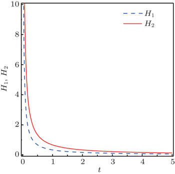
	Fig. 1. Evolution of Hubble parameters H1 = Ȧ(t)/A(t) and H2 = Ḃ(t)/B(t), where m = 2, , and .

Fig. 2.

	Figure Option ViewDownloadNew Window
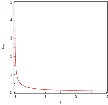
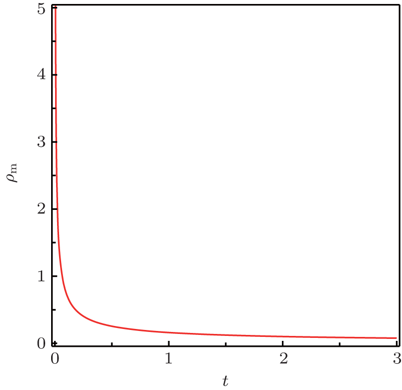	Fig. 2. Evolution of the density ρm in Eq. (39), where m = 2, , , and .

Fig. 3.

	Figure Option ViewDownloadNew Window
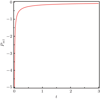
	Fig. 3. Evolution of the pressure Pm1 in Eq. (42), where m = 2, , , and .

Note that we give f (T) in terms of the torsion scalar to explore f (T) in its usual form. But all the calculations in this work are performed using the time dependent form (38). Equation (46) reduces to the isotropic case when m = 1.^[32] For the anisotropic case, f (T) can represent CDM when m ≥ 2. Bengochea et al.^[28] have investigated the observational information for the model f (T) = T − α/(−Tⁿ) by using the most recent SN Ia + BAO + CMB^[64–66] data and they found that the values lie in the range n ∈ [0.23,0.03]. When m = 3, the behavior of f (T) given by Eq. (46) will be generally coincident with that of Ref. [29].

Fig. 4.

	Figure Option ViewDownloadNew Window
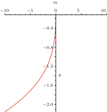
	Fig. 4. Behavior of the deceleration parameter. It is important to note that the parameter m must not take the values −1 and −1/2.