


A new traffic model on compulsive lane-changing caused by off-ramp
[Liu Xiao-He2, Ko Hung-Tang3, Guo Ming-Min1, †,  , Wu Zheng1]
, Wu Zheng1]
|
|


† Corresponding author. E-mail:
Project supported by the National Natural Science Foundation of China (Grant Nos. 11002035 and 11372147).
In the field of traffic flow studies, compulsive lane-changing refers to lane-changing (LC) behaviors due to traffic rules or bad road conditions, while free LC happens when drivers change lanes to drive on a faster or less crowded lane. LC studies based on differential equation models accurately reveal LC influence on traffic environment. This paper presents a second-order partial differential equation (PDE) model that simulates both compulsive LC behavior and free LC behavior, with lane-changing source terms in the continuity equation and a lane-changing viscosity term in the momentum equation. A specific form of this model focusing on a typical compulsive LC behavior, the ‘off-ramp problem’, is derived. Numerical simulations are given in several cases, which are consistent with real traffic phenomenon.
As an important driving behavior, lane-changing behavior (LC) has gained increasing attention in the past few years, and has become a remarkable problem in traffic flow studies. Recent papers revealed that LC is crucial for traffic relaxation[1,2] and safety.[3–7] Therefore, researches on LC problems may carry great significance.
Toledo,[8] Moridpour et al.,[9] and Zheng[10] have reviewed LC, which categorized LC behavior as free LC (i.e., discretionary LC) and compulsive LC (i.e., mandatory LC), according to how the decision of LC is made. Free LC is executed to improve driving conditions, such as changing to a faster lane to achieve higher speed, and changing to a less crowded lane to be more comfortable. Compulsive LC is executed when the driver has to leave the current lane due to certain traffic rules or bad road conditions, for example, the off-ramp problem: a driver who intends to leave the main road from the off-ramp ahead always moves into the right-hand lane or the auxiliary lane in advance to prepare for leaving (in right-driving traffics). This problem is modeled and studied in this paper.
In traffic flow studies, the continuum model is an effective tool and yields good results of studies about how driving behaviors affect the surroundings. Lighthill and Whitham,[11] and Richards[12] respectively originated the model by applying the continuity equation in fluid mechanics to traffic flow, known as the LWR theory. Payne built a second-order continuum model,[13] which has a similar form to the Navier-Stokes equation. Let ρ be the traffic density, u be the speed, then
In the past few years, several continuum traffic models on free LC have been published. Laval and Daganzo adopted the speed difference between adjacent lanes to construct,[7] while Zhu and Wu[18] used the density difference instead. Ko et al.[19] integrated the two forms of the source term to fully characterize the free LC phenomenon. For a section with n lanes, numbered by l = 1,2,…,n from left to right, the continuum equation and momentum equation of Ko et al.’s model are


However, the LC models taking into account both compulsive LC and free LC behaviors rarely appear in the existing literature. This paper presents such a second-order differential equation model, derived based on Ko et al.’s free LC model. The remainder of this paper is organized as follows. In Section 2, a new continuum traffic model addressing compulsive LC and free LC together is derived. In Section 3, a numerical discretization method of the model is given. Numerical results on low-/high-density traffic and non-equilibrium traffic are presented in Section 4. Section 5 summarizes the results in the whole paper, and presents a prospect of further work.
Compulsive LC behaviors affect the density of the surrounding traffic environment, which can be depicted by adding a source term
The vehicles that conduct compulsive LC may have different speeds from the target lane’s average speed, which will change the speed profile nearby, and the free LC momentum equation (
To summarize, for an n-lane road section, the partial differential equation (PDE) traffic model with considering both free and compulsive LC is as follows:
In the off-ramp problem, attraction of the off-ramp ahead is the only considered compulsive LC factor. Thus the compulsive LC source term (namely, the compulsive LC rate)

From the inspection of real traffic phenomenon, we find that the compulsive LC intensity has a general pattern: from the inlet to the upper stream of an off-ramp, the compulsive LC rate keeps increasing up to a peak at some point before the off-ramp, after which it decreases to zero at the point of the off-ramp. This rate then remains zero, because no compulsive LC behavior happens downstream of the off-ramp. According to this inspection, the expression of


 | Fig. 1. Test drawing of |
For the most right-hand side lane (i.e., the one that is adjacent to the auxiliary lane), the value of αn can be determined through the following derivation. The definition of

Let uf be the characteristic speed, ρjam the characteristic density, and L the characteristic length. Let u* = u/uf, ρ* = ρ/ρjam, x* = x/L, t* = t/(L/uf), a* = a/uf, Tr* = Tr/(L/uf), 


The parameter A in Eq. (
We repeate the experiment three times, each lasting half an hour. The number of vehicles passing from the off-ramp is counted and recorded every 5 min. Results are shown in Table
| Table 1. Empirical data for the estimation of A. . |
However, traffic conditions may differ from those of this experiment, depending on the local flow rate, the scale of the studied off-ramp, the average demand for leaving from the off-ramp, and how many lanes that section consists of. Therefore, when using our model for simulation, the value of A should be determined accordingly with reference to our empirical data. For example, in the simulation of the traffic on a two-lane road, the value of A should be half that on a four-lane road, that is, A ∈[20,60] veh/(h·km).
Now we present a numerical simulation method for the model to study the off-ramp problem. The model equations are Eqs. (
The finite difference scheme is designed by referring to Refs. [21] and [22]. Use the forward difference formula for time derivatives, the backward difference formula for spatial derivatives with the coefficient of speed, and the forward difference formula for spatial derivatives with the coefficient of density, then the scheme will be obtained as follows (subscript l is omitted):
When using the discretization scheme for simulation, let dx = 0.05, dt = 0.005, J = 20, and N = 2000, where J and N are the total number of spatial grids and temporal steps respectively. Constants are set to be Tr = 0.02, a = 0.4, 
As for the boundary conditions, let all profiles keep unchanged at the inlet, and use the Neumann condition at the outlet, then we will have

Three numerical cases of the off-ramp problem are studied to demonstrate the reasonability and the applicability in equilibrium and non-equilibrium traffic of our model. Figure
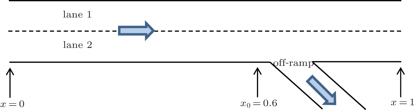 | Fig. 2. Sketch of the off-ramp problem. |
Case 1 is designed to validate the model and the discretization scheme, and also to study LC influence on the traffic environment. Suppose that traffic density is low on both lanes, and the speed and density on both lanes are evenly distributed. The initial conditions are

Equilibrium speed Ue is given by the dimensionless Greenshields speed-density relationship:[23]


Numerical results of the four conditions are drawn in Fig.
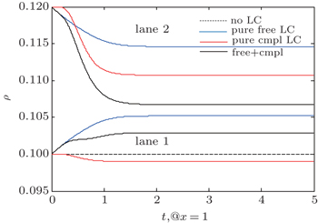
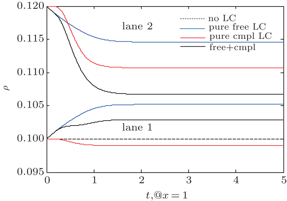 | Fig. 3. ρ–t in low density state. |
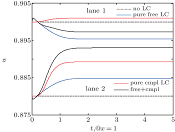
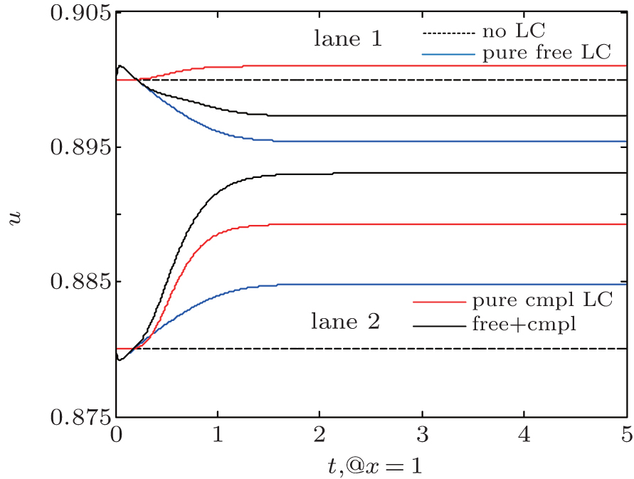 | Fig. 4. u–t in the low density state. |
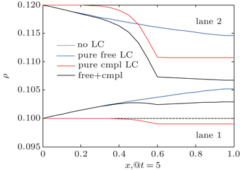
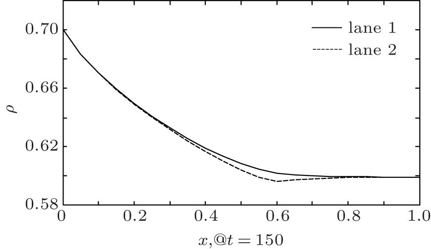
 | Fig. 5. ρ–x in low density state. |
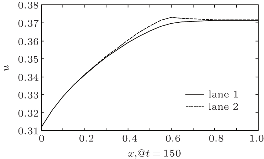
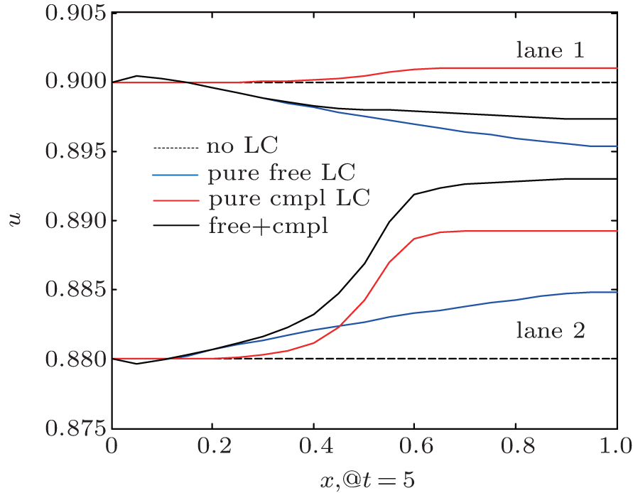 | Fig. 6. u–x in low density state. |
Figures
Then figures
It is shown in this case that our model simulates traffic with free and compulsive LC well at low density, and the pure free LC case yields the same results as the low density case in Ref. [19] (at medium and high density, our results of the pure free LC case agree with those in Ref. [19] as well). Two kinds of LCs show different influence patterns in the traffic state. The discretization scheme is stable, and the parameters are well set so as to obtain reasonable results.
The model (


Figures
 | Fig. 7. ρ–x in medium density state. |
 | Fig. 8. u–x in medium density state. |
The high-density state usually exists in congested urban traffic, where almost every space available is occupied and the speeds and densities of the two lanes are very close. Thus the initial conditions for the high-density state are given as

Figures
 | Fig. 9. ρ–x in high density state. |
 | Fig. 10. u–x in high density state. |
Figures
Generally speaking, a second-order differential equation model can simulate the non-equilibrium traffic state well. Therefore, we design Case 3 to study our model in a non-equilibrium state simulation. Take the same settings as the free + compulsive LC condition in Case 1, except that the inlet boundary condition (
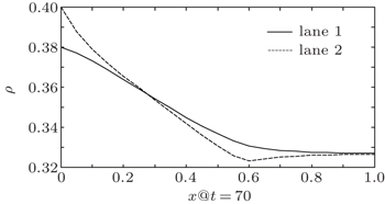
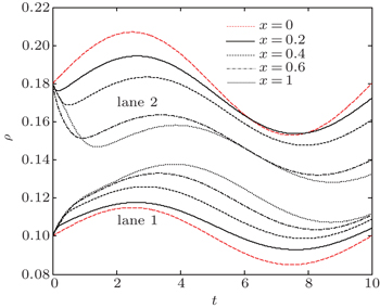
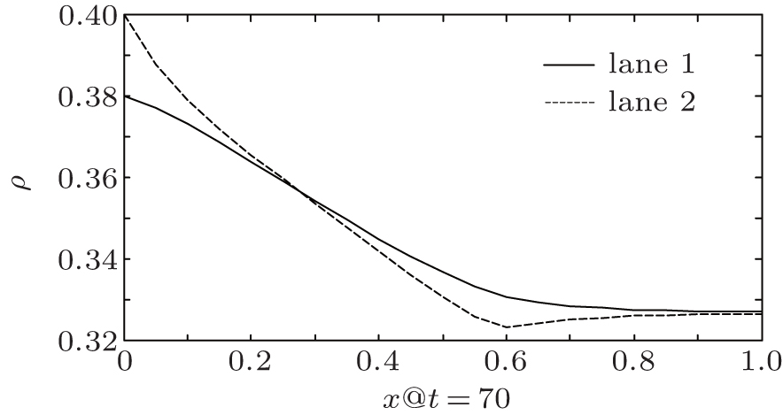
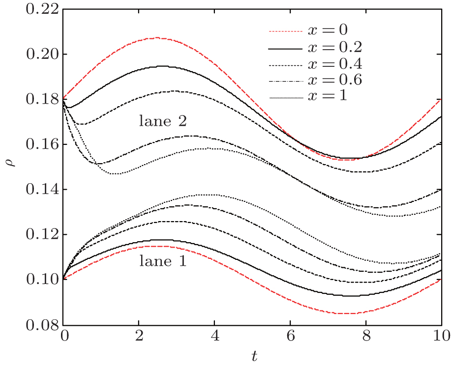 | Fig. 11. ρ–t in non-equilibrium state. |
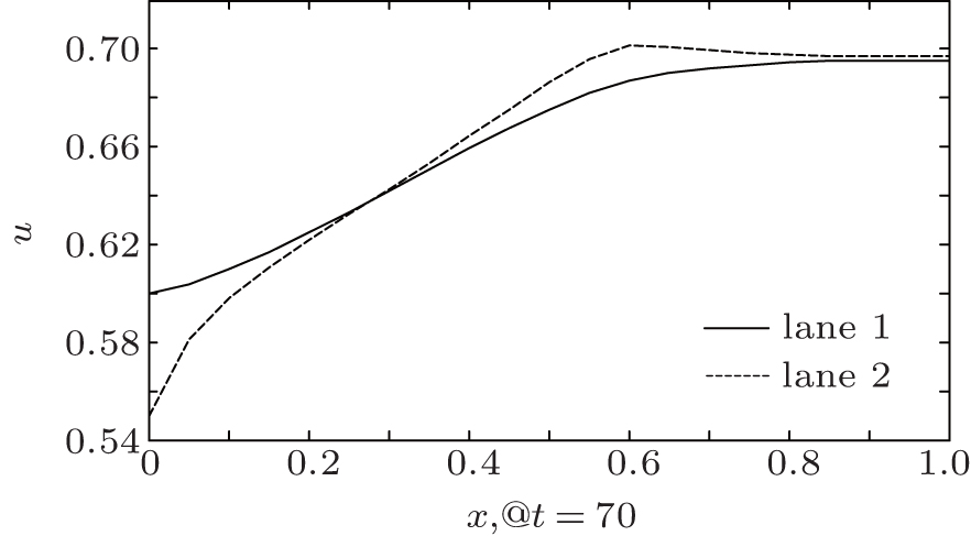
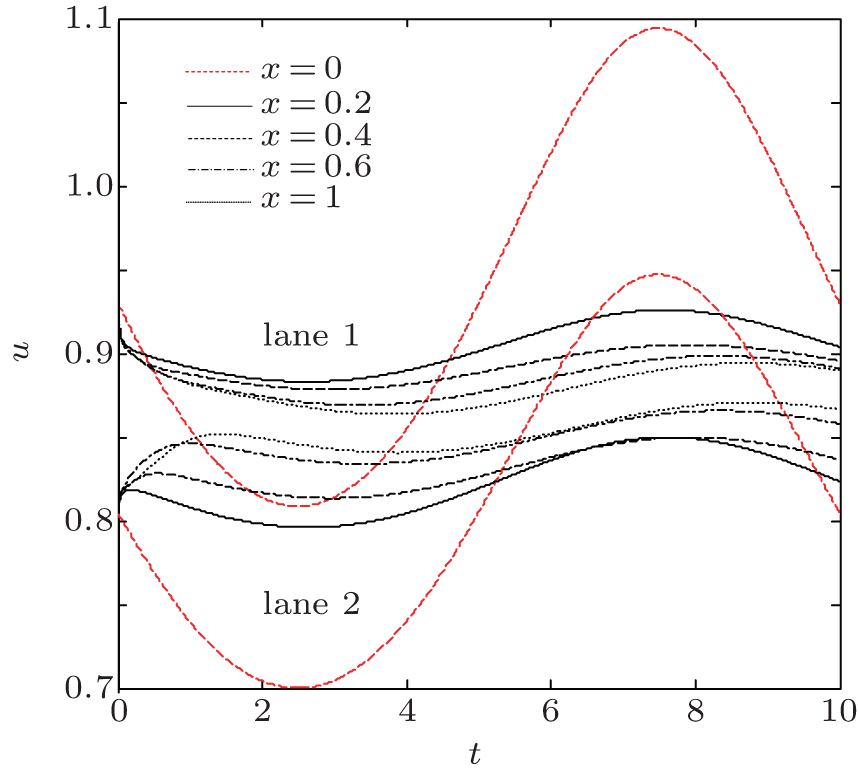 | Fig. 12. u–t in non-equilibrium state. |
It can be seen in the figures that as the phase of the fluctuation at the inlet moves downstream, the amplitude reduces. This is caused by the free LC, which is in accordance with the second case from Ref. [19]. On the other hand, at x = 0.4, x = 0.6, and x = 1 respectively, an overall trend that density drops and speed increases can be seen, with the scenario at x = 0.6 being the most evident. This is caused by the compulsive LC, which brings down the traffic flow of the road section. This case validates the applicability of our model in the simulation of non-equilibrium traffic near an off-ramp.
In this paper we establish a new second-order continuum traffic model with the consideration of both free LC and compulsive LC behaviors. For the off-ramp problem, we give a form of the source term of compulsive LC, and determine its value range of the parameter by the empirical data taken from an off-ramp at Shanghai. A discretization scheme for our model is constructed and applied to three numerical cases, which show that the proposed model and discretization scheme can provide reasonable simulations for various traffic states.
The compulsive LC function model is logically derived through the inspection of real traffic, however, we are interested in looking into how this model can be verified and how the parameters could be determined through empirical data in the future.
In this paper, only one kind of compulsive LC is discussed. However, other kinds of compulsive LC behaviors exist, such as the keep-right-except-to-pass-rule problem: under certain traffic rules, drivers have to change back to the slow lane after overtaking the car in front of it by using the quick lane.[24,25] Such a situation may be simulated by proposing another suitable Φramp,n term in Eq. (
| 1 | |
| 2 | |
| 3 | |
| 4 | |
| 5 | |
| 6 | |
| 7 | |
| 8 | |
| 9 | |
| 10 | |
| 11 | |
| 12 | |
| 13 | |
| 14 | |
| 15 | |
| 16 | |
| 17 | |
| 18 | |
| 19 | |
| 20 | |
| 21 | |
| 22 | |
| 23 | |
| 24 | |
| 25 |