Computational analysis of the roles of biochemical reactions in anomalous diffusion dynamics
Rueangkham Naruemon1, Modchang Charin1, 2, 3, †,
Biophysics Group, Department of Physics, Faculty of Science, Mahidol University, Bangkok 10400, Thailand
Centre of Excellence in Mathematics, CHE, 328, Si Ayutthaya Road, Bangkok 10400, Thailand
ThEP Center CHE, 328 Si Ayutthaya Road, Bangkok 10400, Thailand


† Corresponding author. E-mail: charin.mod@mahidol.edu

Project supported by the Thailand Research Fund and Mahidol University (Grant No. TRG5880157), the Thailand Center of Excellence in Physics (ThEP), CHE, Thailand, and the Development Promotion of Science and Technology.

Abstract
Abstract

Most biochemical processes in cells are usually modeled by reaction–diffusion (RD) equations. In these RD models, the diffusive process is assumed to be Gaussian. However, a growing number of studies have noted that intracellular diffusion is anomalous at some or all times, which may result from a crowded environment and chemical kinetics. This work aims to computationally study the effects of chemical reactions on the diffusive dynamics of RD systems by using both stochastic and deterministic algorithms. Numerical method to estimate the mean-square displacement (MSD) from a deterministic algorithm is also investigated. Our computational results show that anomalous diffusion can be solely due to chemical reactions. The chemical reactions alone can cause anomalous sub-diffusion in the RD system at some or all times. The time-dependent anomalous diffusion exponent is found to depend on many parameters, including chemical reaction rates, reaction orders, and chemical concentrations.

1. Introduction

Diffusion is likely to be the most important transportation process inside a living cell. However, the cell cytoplasm is not a simple solvent; it is crowded and consists of many chemically reactive molecules. Therefore, various factors can hinder diffusion in living cells.[1,2] In particular, the chemical reactions or biochemical conversions in metabolic and signal transduction pathways can affect the cellular transportation processes.[1,3] In general, the reaction diffusion processes in a living cell can be described by a set of reaction–diffusion equations,

where ci(r,t), Di, and Ri are the concentration, diffusion constant, and reaction term of the i-th substance, respectively. For systems in which particles or molecules diffuse freely via Brownian dynamics, the mean-square displacement (MSD) of the particles increases linearly with time. Some researchers also hold that this reaction diffusion process can be investigated under the assumption of Brownian or normal diffusion.[4,5] However, a number of recent experimental studies based on single-particle tracking (SPT) and fluorescence correlation spectroscopy (FCS) mapped out the intracellular molecules’ trajectories to determine the relationship of MSD with time and revealed that the diffusions in cells and on cell membranes are often anomalous.[69] This was initially suggested by the experimental results of Cajal bodies in the nucleus of HeLa cells.[10] Two other notable studies of the discovery of anomalous sub-diffusion in living cells were the diffusion of telomeres in the nucleus of mammalian cells and the diffusion of protein in HeLa cells and polytene cells of Drosophila larval salivary glands.[11,12] It was reported that the diffusions in different cell types cause different anomalous diffusions and the anomalous behavior of intracellular diffusion can be presumably the result of the obstruction of molecular crowding in the cytoplasm as well as chemical kinetics.[1,3,6,13,14] However, the experimental data on diffusion in living cells are difficult to identify what factors exactly cause the anomalous diffusion within cells. Therefore, theoretical and simulation studies are necessarily required to add more understanding of diffusion and transport mechanisms of biological processes in living cells.

Anomalous diffusion is characterized by the MSD of diffusing particles, which grows with the power law of time:

where α represents an anomalous diffusion exponent that indicates the diffusion behavior.[15] If α > 1, the diffusion process is characterized by super-diffusion, whereas α =1 corresponds to normal diffusion.[1,13,16] Anomalous sub-diffusion occurs when 0 < α < 1 and has been found in many intracellular systems.[3,6] However, the underlying physical or chemical causes of anomalous sub-diffusion in cells are not fully understood.[1,3]

The ability of chemical reactions to cause anomalous sub-diffusion has not yet been experimentally investigated. However, it has been observed and clearly identified in many other cases. Many researches demonstrated that the continuous time random walk (CTRW) model is one of the most successful theoretical models of anomalous diffusion.[13,17,18] Also theoretical models based on the CTRW and fractional reaction–diffusion equations confirmed that chemical components can cause anomalous sub-diffusion.[13,17,1923] Likewise, Haugh used the framework of Green’s function analysis to demonstrate that the reaction diffusion mechanism could not be assumed to be normal diffusion.[3] Using Monte Carlo simulations on a simple lattice model, Saxton also showed that the binding mechanism alone can cause anomalous diffusion at some or all times.[24] In addition, by using lattice gas automata, researchers have recently found that the diffusion in the Michaelis-Menten mechanism exhibits anomalous diffusion in a transient period.[25,26]

In this work, we further investigate the diffusive anomaly of a reaction diffusion system by using MCell, a 3D spatially realistic Monte Carlo simulator that tracks individual molecules.[27] Although the MCell program has been optimized for Monte Carlo simulation, a deterministic approach is computationally more efficient and easier to implement for most problems. Thus, we propose alternative methods using a deterministic algorithm to investigate the anomalous behaviors in reaction diffusion systems which have been numerously elucidated by stochastic simulation in published versions. The effects of reaction rate and reaction type on the diffusion behavior are also investigated.

2. Materials and methods

Reaction–diffusion equations are a mathematical model that explains the changes of one or more substances in space and time in chemical reaction and diffusion processes. In addition to the study of chemistry, these equations can also be used to describe many intracellular processes.[28,29] In the present work, we study a Ca2+ buffering system in cells. This Ca2+ buffering system can control various processes, including neurotransmitter release during synaptic transmission. The calcium buffering dynamics can be written in the form of a chemical equation as follows:

where Bi and CaBi represent the free buffers and calcium bound buffers, respectively, and i = s or m represents stationary or mobile buffer, respectively.[5] In our model, an initial number of Ca2+ ions are released in the center of an unbounded space, where either mobile or stationary buffers are homogeneously distributed.

2.1. Monte Carlo simulations

We investigate anomalous diffusion in the Ca2+ buffering system by using MCell version 3.1, a Monte Carlo (MC) algorithm that tracks individual molecules.[27] The MCell simulations are performed in three-dimensional (3D) space, and all of the Ca2+ trajectories are recorded during the simulations. The recorded trajectories are then used to calculate the mean squared displacement (MSD) of Ca2+. In all simulations, the dimensions of the computational geometry are 4 μm × 4 μm × 4 μm. Initially, 54902 ions of Ca2+ are held in a spherical shell with a radius of 7.5 nm located at the origin and are then released at time t = 0, whereas 549020 ions of buffers are uniformly distributed throughout the computational box. These numbers of ions correspond to a calcium concentration of 1.425 μM and a buffer concentration of 14.25 μM in our computational domain. All surfaces of the computational box are reflective to all molecules. To study only the reaction diffusion dynamics and avoid the possible effects of the boundary on calcium ion dynamics, we ensure that calcium ions and calcium bound buffers do not reach the boundaries of our computational box. All parameter values used in MCell simulations are adjusted to reduce the simulation time, as given in Table 1.

2.2. Deterministic simulations

Deterministic simulation is an alternative approach to the study of the diffusive behaviors in the system in order to obtain longer time courses of the MSD. Assuming mass action kinetics and Fickian diffusion, the concentration changes in Eq. (3) are then calculated by using the following partial differential equations:

where DCa, DBi, and DCaBi are the diffusion constants of free calcium, free buffers, and Ca2+ bound buffers, respectively, and and are the association and dissociation rate constants for buffer i, respectively. In deterministic simulations, we treat the computational space as a visual one-dimensional infinite system, within which the initial pulse of Ca2+ is released as the Dirac delta function ([Ca2+]0 = δ(x)) and buffers initially distributed homogeneously. The reaction diffusion equations in Eq. (4) are solved by using the explicit finite different algorithms in MATLAB. The numerical values of the parameters used in the deterministic model are shown in Table 1.

Table 1.

Parameter values in the simulated system.

.
2.3. Calculations of MSD from deterministic simulations

The deterministic calculations that solve the differential equations in Eq. (4) can yield probability density functions (PDFs) at different times. In this work, the PDFs will be used to estimate the relationship between MSD and time. The MSD of Ca2+ is estimated from either the half width at half maximum (HWHM) or numerical integration of the PDFs. Both MSD estimation methods are generic and can be used with any PDFs. In the first method, the shape of the PDF is characterized by the HWHM value. This approach has previously been used to investigate anomalous diffusion as described in Sagi, et al.’s work.[31] The HWHM is estimated in MATLAB using the linear interpolation function, interp1, which requires at least two known data points. The syntax of interp1 is interp1 (x, y, xi), where x is a vector that contains independent variable data, y is a vector that contains dependent variable data and xi is the array of data points to be interpolated.

For the integration method, the MSD (〈x2〉) can be directly calculated from definition,[32]

where P(x,t) is a PDF. The equation is numerically integrated using the trapezoidal rule.

2.4. Chemical reaction orders

Different types of reactions are investigated to systematically study the effects of reactions in reaction diffusion systems.

3. Results and discussion
3.1. Mote Carlo simulations of reaction diffusion systems

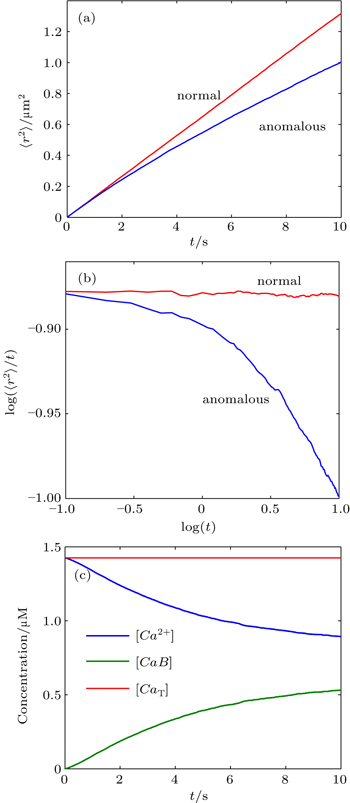
First, we used MCell, a particle-based Monte Carlo algorithm, to investigate anomalous diffusion in reversible bimolecular reaction, which can be found in most living cells. The particle trajectories in three-dimensional space are recorded and used to calculate their mean squared displacement (MSD or 〈r2〉) as shown in Figs. 1(a) and 1(b). Figure 1 shows 〈r2〉 as a function of time, obtained from the free diffusion system and a reaction diffusion system that exhibits anomalous diffusion. The distinction between normal diffusion and anomalous diffusion becomes more apparent when the data are plotted as log (〈r2〉/t) versus logt as shown in Fig. 1(b). Because the slope of the straight line in Fig. 1(b) is α − 1, normal diffusion produces a horizontal line, which corresponds to α = 1. The result shows that the anomalous diffusion exponent is not constant (see more results in Section 3). To avoid boundary effects, the box size must be sufficiently large to prevent calcium ions and calcium-bound buffers from reaching the surfaces of the box. This constraint causes the simulations to require a very long time to reach the steady state. Obtaining 10 s of the simulation result in Fig. 1 requires 9 h of computational time, and the reaction still does not reach a steady state as shown in Fig. 1(c). Hence, determining the long-time MSD from a particle-based stochastic simulation is impractical from a time standpoint. To reduce simulation time, the deterministic algorithm will be used for further analyses.

Fig. 1. (a) Monte Carlo results for the mean-square displacement, 〈r2〉, as a function of time, t, for free diffusion (normal) and reaction diffusion (anomalous) in a linear plot. (b) Monte Carlo MSD is plotted as log (〈r2〉/t) versus logt. The slope of a straight line in this plot is α − 1; thus, normal diffusion dynamics yields a horizontal line. (c) The concentrations of the reactant, (Ca2+), and product, (CaB), as a function of time. The total calcium concentration, (CaT), is also shown.
3.2. Relationship between MSD and HWHM

We cannot track the movement of individual molecules in the deterministic simulation; thus, the MSD cannot be directly computed from particle trajectories, and an alternative method to compute the MSD becomes necessary. We propose two alternative approaches to extract the MSD from the PDFs. In the deterministic calculations, we obtain PDFs at different times (P(x,t)) by solving the differential equations in Eq. (4). The PDFs at each time point could then be analyzed to extract the MSD by using numerical interpolation for HWHM and numerical integration methods as described in the part about the methods in Section 2.

For the free diffusion in an infinite system with an initial [Ca2+] given by the Dirac delta function, the PDF can be written in the form of a Gaussian function[34] as verified in Fig. 2(a). The general Gaussian form f (x) = A exp(−x2/2σ2), where A is the amplitude and σ is the standard deviation,[4] can be utilized to determine the relationship between the MSD and the HWHM because f (HWHM) = A exp(−HWHM2/2σ2) = A/2. This calculation yields We also know that the MSD, 〈x2〉, is the variance of the Gaussian distribution, σ2, which grows linearly with time, i.e., σ2 = 2Dt.[34] Thus, HWHM2 = 2 ln 2〈x2〉. In n-dimensional space, this relationship can also be generalized to the following expression:

However, the PDF of a reaction diffusion system cannot be characterized by the Gaussian PDF as shown in Fig. 2(b). In fact, the non-Gaussian forms of PDF in reaction diffusion systems are quantitatively different because different mechanisms, e.g., different reaction orders, lead to different PDFs as indicated in many researches.[13,1820] Hence, its general form has not yet been found, although many approaches have been introduced to elucidate the PDFs of anomalous dynamics.[1,18,35] An explicit relationship between the MSD and the HWHM is lacking for this case. Therefore, in this study Mote Carlo simulations are used to numerically determine the relationship between the HWHM and the MSD for the reaction diffusion process. The MSD is directly calculated from individual particle trajectories, and the HWHM is estimated from the corresponding [Ca2+] curves. We find that the MSD of a reaction diffusion system remains linearly proportional to HWHM2 as shown in Fig. 3; hence, equation (2) yields HWHM2tα.

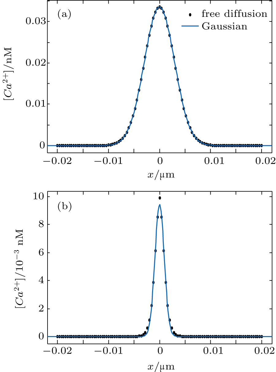
Fig. 2. The [Ca2+] at t = 2 s (dots) are fitted to a Gaussian function (solid curves) for (a) free diffusion with the goodness of fit r-squared = 1 and (b) reaction diffusion with the goodness of fit r-squared = 0.997.
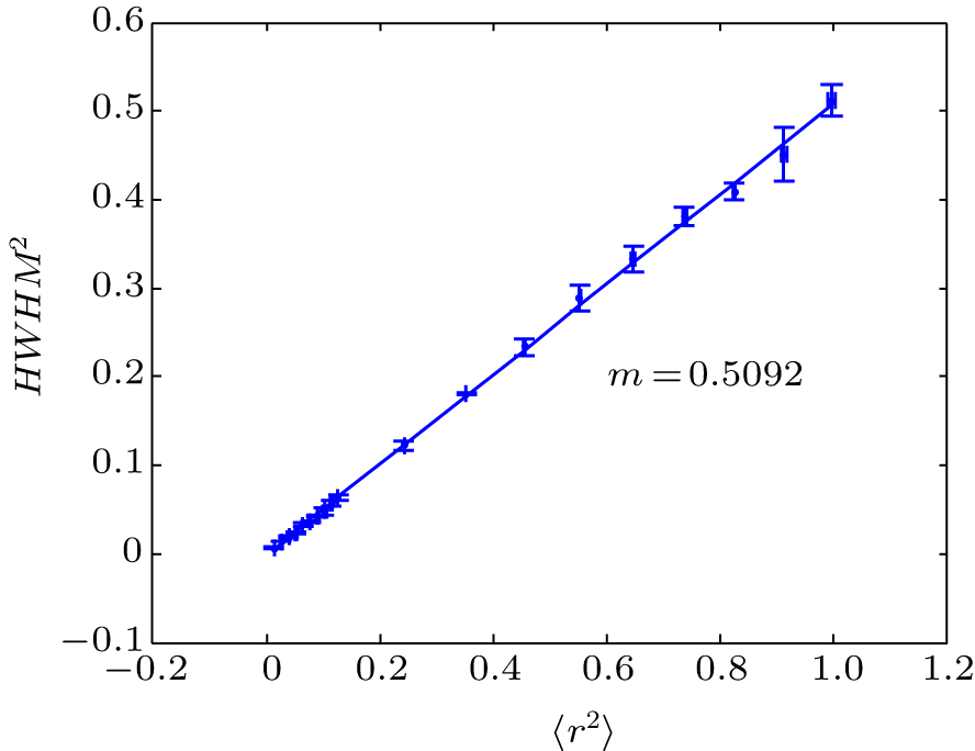
Fig. 3. Relationship between HWHM2 and MSD (〈r2〉) in the reaction diffusion system. Simulation conditions and parameters are the same as those in Fig. 2(b).

The MSD values obtained from HWHM interpolation and numerical integration for normal and anomalous diffusion are compared in Figs. 4(a) and 4(b), respectively. We find that the HWHM interpolation method results in some fluctuations for both normal (free diffusion) and anomalous (reaction diffusion) cases. This error may be due to the linear interpolation between two nearest data points. If the data points are more distant, the interpolation method yields a larger error. Therefore, we henceforth investigate anomalous diffusion dynamics in the reaction diffusion system using deterministic algorithms and the integration method to extract the MSD from the PDF.

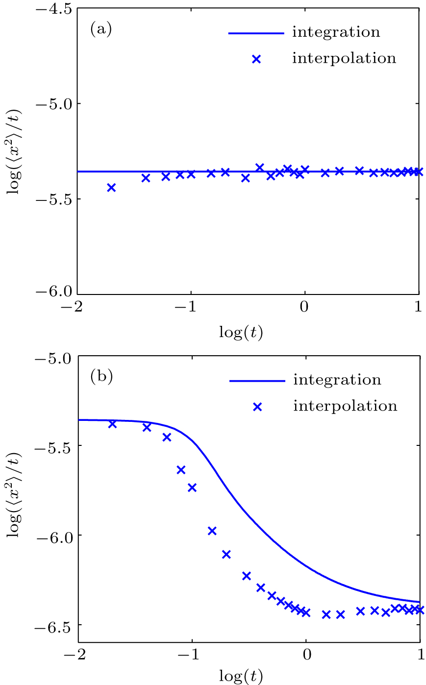
Fig. 4. Comparisons between the MSD obtained from HWHM interpolation and that from numerical integration method for (a) normal diffusion and (b) anomalous diffusion.
3.3. Effects of the concentration and diffusion coefficient of the buffer

The reaction diffusion dynamics is henceforth investigated in one-dimensional space by using deterministic simulations in MATLAB. To study the anomalous behaviors of the system, the anomalous diffusion exponent (α) in the equation 〈x2〉 = Γtα is computed. As described above, the numerical integration method is selected to investigate the dynamics of reaction diffusion mechanisms and analyze the anomalous diffusion exponents (α). In this section, we focus on the reversible reaction of the Ca2+ buffering system. We investigate the effects of buffer concentration and diffusion coefficient on the diffusive behavior of Ca2+ in a buffer solution; the parameter values for this system are shown in Table 1.

Figure 5(a) shows the time courses of MSD plotted as log(〈x2〉/t) versus logt for different buffer concentrations and diffusion coefficients. Because the slope of the straight line in this figure is α − 1, normal diffusion yields a horizontal line. This figure indicates that the diffusion of reversible bimolecular reaction is characterized by three time regimes. The diffusion is normal at early times and then rapidly changes to anomalous diffusion at an intermediate time. The diffusion subsequently becomes normalized when the dynamics reaches a steady state as illustrated in Figs. 5(a) and 5(b). However, the normal diffusion period is shorter at early time points for higher reaction rates.

Fig. 5. (a) Plots of log (〈x2〉/t) versus logt for Ca2+ in the presence of either stationary or mobile buffer at [Bi]0 = 2.64 μM and 26.4 μM; (b) time evolutions of Ca2+ and Ca2+-bound buffers (CaB) concentrations, where [Bm]0 = 26.4 μM, and the total calcium concentration (CaT) is also shown; (c) plots of the instantaneous anomalous diffusion exponent (αins) versus logt, for different values of [Bm] and [Bs].

Because the MSD can be expressed as
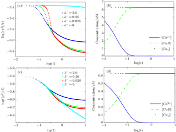
where Γ is a constant, the value of α can be obtained from the slope of the plot of log(〈x2〉/t) versus logt. The results in Fig. 5(a) suggest that α is not constant over time. Therefore, we calculate the instantaneous anomalous exponent (αins), an anomalous diffusion exponent during an infinitesimal time interval as shown in Fig. 5(c). Two major transitions, from α = 1 at early times to α < 1 at intermediate times and a return to α = 1 again at late times, are clearly evident, which suggests that the diffusion in reversible bimolecular reactions follows transient anomalous sub-diffusion. Furthermore, figure 5(a) also shows that the duration of the anomalous period increases and the diffusion is more anomalous if we either increase the buffer concentration or reaction rate or reduce the diffusion coefficient of buffers.

3.4. Effects of dissociation rate and reaction order

Figure 6(a) shows the time courses of MSD for Ca2+ diffusion in mobile buffers and different dissociation rates (k) and constant association rates (k+). The values of other parameters used in this simulation are shown in Table 1. We find that the reversible second-order reaction usually exhibits more anomalous diffusion in the intermediate time regime as the dissociation rate (k) decreases. The overall dynamics continues to follow the transient anomalous sub-diffusion, similar to the results in Section 3. At high values of t when the reaction reaches a steady state, the diffusion reverts to the normal diffusion. However, if k approaches to zero, the reaction becomes an irreversible second-order reaction, with a rate r = k+[Ca2+][Bm]. In this case, diffusion remains normal until the Ca2+ concentration is extremely close to zero at very high values of t as shown in Figs. 6(a) and 6(b). This result is expected because the parameter values in Table 1 indicate that [Bm]0 ≫ [Ca2+]0; thus, the concentration of mobile buffers can be considered to be constant and r = k+[Ca2+][Bm] = k′[Ca2+], where k′ = k+[Bm] is constant. Therefore, the second-order reaction reduces to a pseudo-first order reaction in this case, which results in normal diffusion.[31]

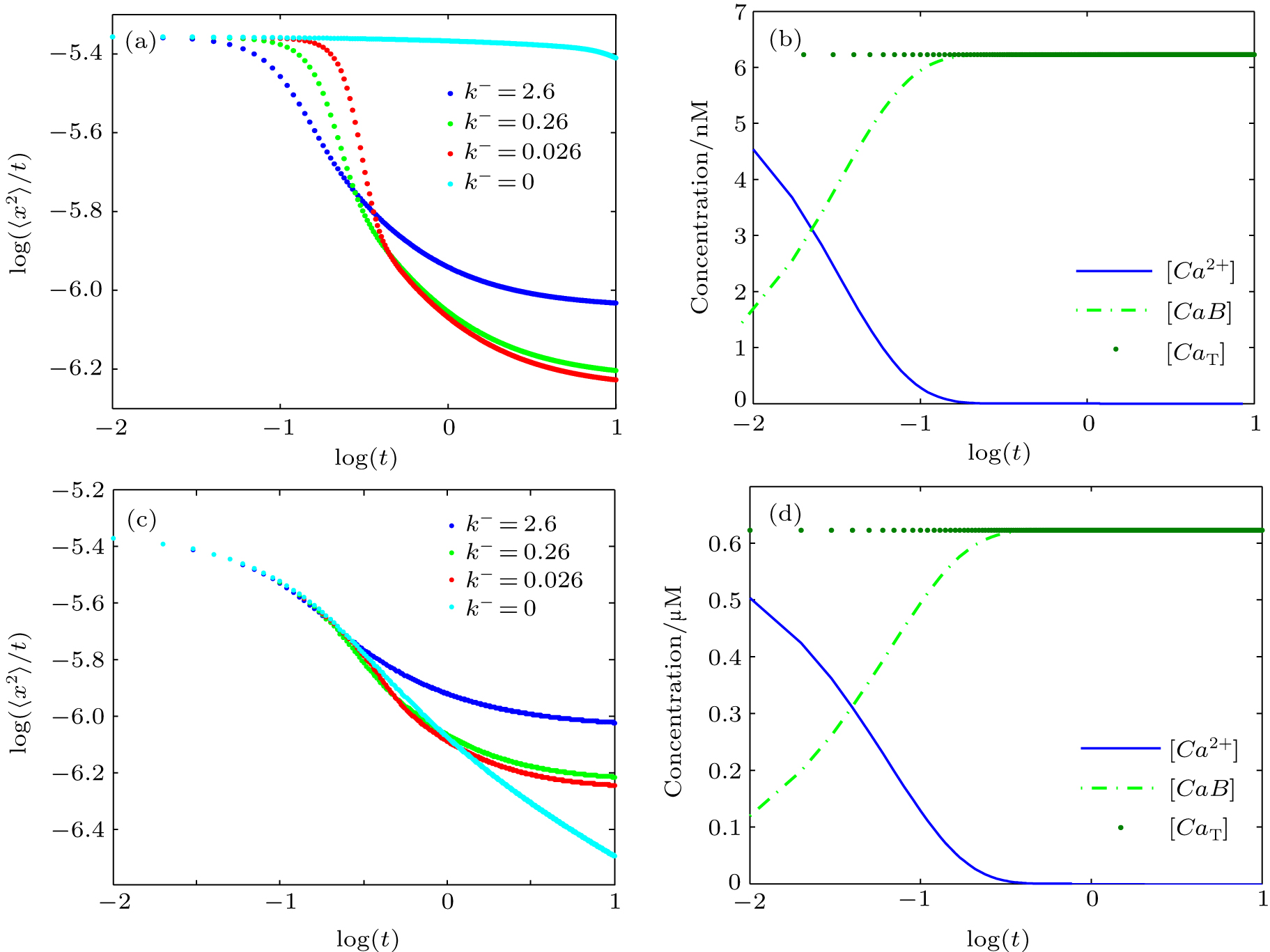
Fig. 6. (a) Plots of log (〈x2〉/t) versus logt for various values of dissociation rate (k) in the case of calcium diffusion in mobile buffers at [Bm]0 = 26.4 μM and [Ca2+]0 = 6.23 nM; (b) concentration changes of Ca2+, CaBm, and CaT for k = 0; (c) plots of log(〈x2〉/t) versus logt for various values of dissociation rates (k) in the case of calcium diffusion in mobile buffers at [Bm]0 = 26.4 μM and [Ca2+]0 = 0.623 μM; (d) time-dependent concentration variations of Ca2+,CaBm, and CaT for k = 0.

To demonstrate the effect of the initial Ca2+ concentration, we also change [Ca2+]0 to 0.623 μM. The results in Fig. 6(c) show that the magnitudes of k− and the slope in the anomalous region inversely correlate. Generally, reducing the dissociation rate exacerbates the anomalous nature of the diffusion. The diffusion remains anomalous even when k = 0, unlike the case when [Ca2+]0 = 6.23 nM (see Fig. 6(a)). Moreover, an irreversible second-order reaction and k = 0 result in an anomalous sub-diffusion throughout the simulation time, even when the Ca2+ concentration reaches very low values at very late times as shown in Fig. 6(d).

For the first-order reaction the reaction diffusion dynamics is governed by

where k+ and DCa are constants. In this case, we can analytically show that the diffusion dynamics of Ca2+ is normal at all times. Now we write the [Ca2+] in the following form:

where C0 (x,t) is a function. Substituting Eq. (8) into Eq. (7), we then obtain a condition for C0(x,t),

This implies that C0(x,t) is a solution of the diffusion equation. Therefore, the corresponding solution of the first-order reaction diffusion equation with the initial condition C(x,0) = δ(x) is in the form of the Gaussian function multiplied by the exponential function of time. At a particular time, this exponential function exp(−k+t) does not change the shape of the Gaussian function, except its height. Thus the MSD of Ca2+ in the first-order reaction diffusion process is not affected by the reaction. Therefore Ca2+ shows normal diffusion at all times. This analytical result agrees well with our computational result shown in Fig. 7 (solid line). The time evolutions of the MSD and the values of instantaneous anomalous diffusion exponent (αins) for different reaction types are summarized in Figs. 7(a) and 7(b), respectively. This figure shows that different types of reactions result in different diffusion dynamics.

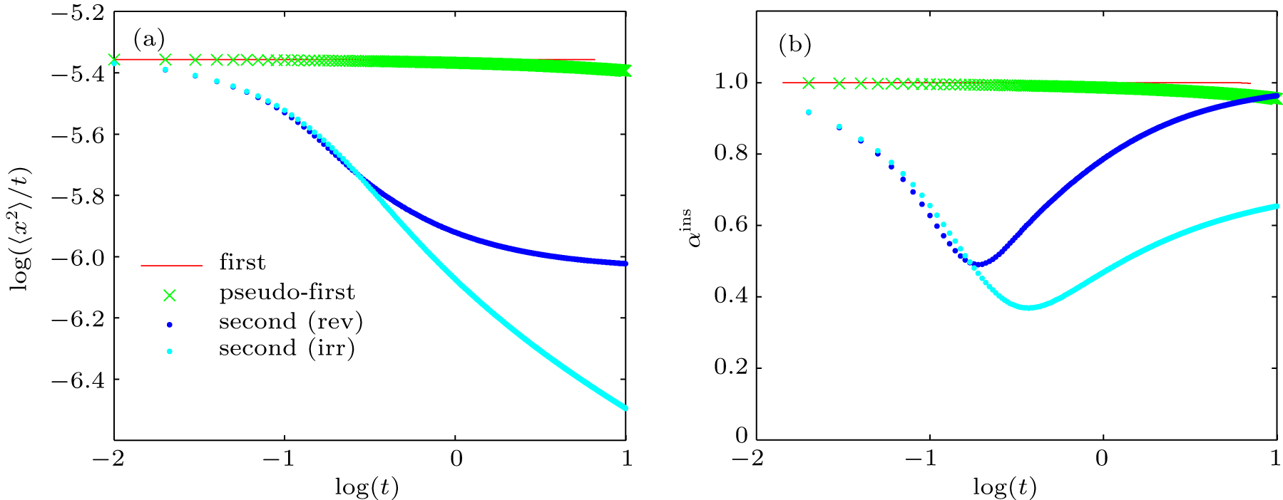
Fig. 7. Time evolutions of (a) MSD and (b) instantaneous anomalous diffusion exponents (αins) for different types of reactions.
3.5. Average anomalous diffusion exponent in the period of anomalous sub-diffusion

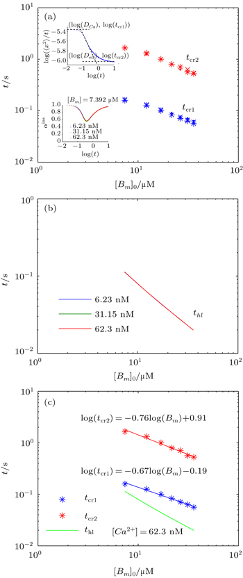
To calculate the average anomalous diffusion exponent (αavr) in the period of anomalous sub-diffusion, we first find crossovers between normal and anomalous diffusion by plotting log(〈x2〉/t) versus log(t). As shown in previous sections, in the case of a reversible second-order reaction, there are two major transitions at short time and at long time respectively. At the first crossover (x1,y1) diffusion changes from normal to sub-diffusion and at the second crossover (x2,y2) diffusion changes from sub-diffusion to normal diffusion again. To find these crossovers, we locate the intersections between two straight lines in anomalous and normal regions at early time and at long time as shown in the upper inset of Fig. 8(a). This yields (x1,y1) = (logtcr1,logDCa) and (x2,y2) = (logtcr2,logD(∞)) where tcr1 and tcr2 are the first and second crossover time, respectively, and D(∞) is an effective diffusion coefficient of calcium at very long time.[6] Figure 8(a) shows the graphs of tcr1 and tcr2 each as a function of buffer concentration for various calcium concentrations. It indicates that tcr1 and tcr2 are insensitive to the change of the initial Ca2+ concentration. This also corresponds with the result of αins with [Ca2+] varying as shown in the lower inset of Fig. 8(a).

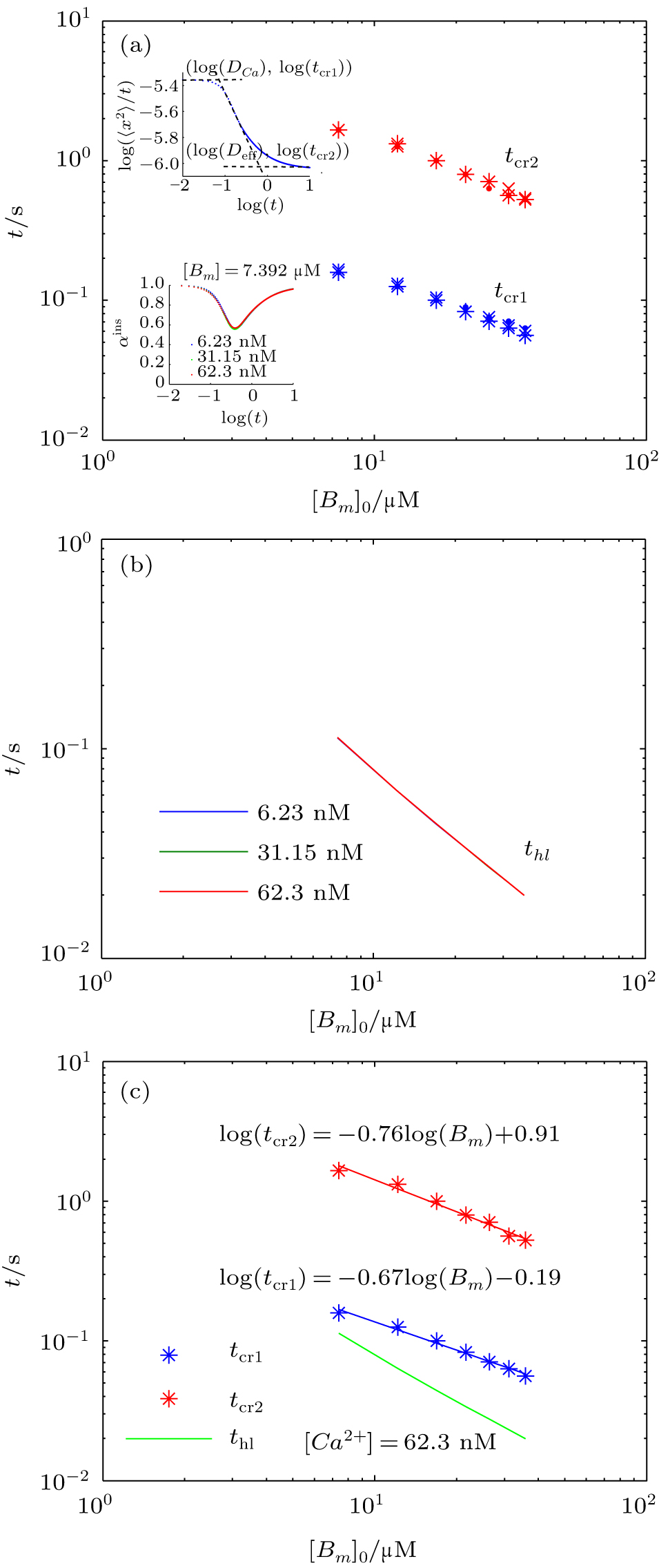
Fig. 8. (a) The first and second crossover time (tcr1, tcr2) each as a function of mobile buffer concentration at three different concentrations of calcium ions: [Ca2+]0 = 6.23,31.15,62.3 nM (note the overlap of data points for different values of [Ca2+]0), for k+ = 1 and k = 2.6. The upper inset in panel (a) shows the intersections of the lines yielding the crossover times, tcr1 and tcr2. The lower inset shows αins for different values of [Ca2+]0. (b) The calcium half-life obtained from Eq. (10) at the same [Ca2+]0 as that in panel (a). (c) Plots of tcr1 and tcr2 in comparison to thl obtained from the analytic solution in Eq. (10).

To get an insight into tcr1 and tcr2, we calculate the half-life of calcium concentration in a well-mixed condition where both calcium and buffer are uniformly distributed. For the reversible bimolecular reactions,

the half-life of Ca2+ (thl) is found to be as follows (see Appendix A, for detailed description of the derivation):

where

k = k/k+; [Ca2+]0; and [B]0 are the initial concentrations of calcium and buffer, respectively. The calcium half-life calculated from Eq. (10) demonstrates that it is insensitive to the change of initial Ca2+ concentration (Fig. 8(b)), which is consistent with the crossover times (tcr1 and tcr2) in Fig. 8(a). Furthermore, it also shows that the tcr1 is relatively close to the thl as illustrated in Fig. 8(c). Therefore, the change from normal to sub-diffusion occurs when the calcium concentration is reduced by about half of its initial concentration. It is noticeable that the tcr1, tcr2 and thl are all involved with the buffer concentrations in power-law relations. We also find that tcr1, tcr2, and thl are all insensitive to the change of dissociation rate k (Fig. A1).

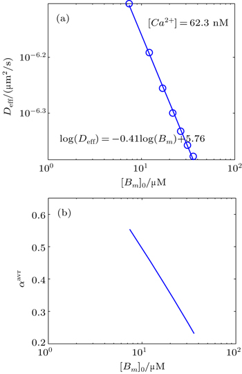
Likewise, we obtain the calcium effective diffusion coefficient Deff (or D(∞)), from the simulation results as plotted in Fig. 9(a). The value of αavr in the anomalous sub-diffusive region can be then calculated from the slope of the graph of log(〈x2〉/t) versus logt. Consequently, we obtain the empirical form of αavr as a function of buffer concentration as follows:

The values of αavr in the period of anomalous sub-diffusion are illustrated in Fig 9(b).

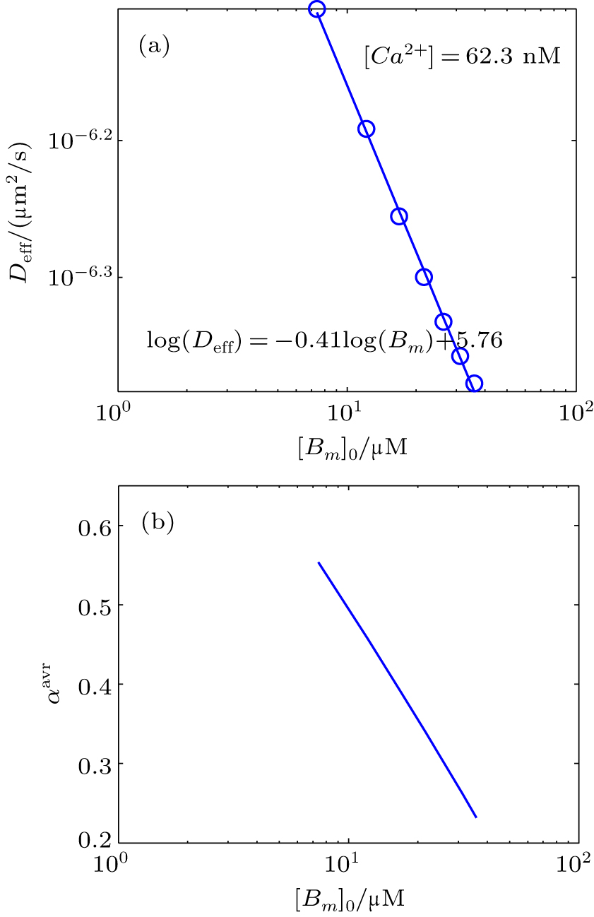
Fig. 9. (a) Plot of the effective diffusion coefficient (Deff) as a function of initial mobile buffer concentration [Bm]0. (b) The value of αavr in the period of anomalous sub-diffusion calculated from Eq. (11).
4. Conclusions

In this work, the roles of biochemical reactions in diffusion dynamics are computationally investigated by using both deterministic and stochastic algorithms. Because we cannot track individual particle trajectories in the deterministic simulations, methods to estimate the MSD from deterministic calculations are also investigated. We find that the numerical integration of the PDF best estimates the MSD. Computational and theoretical analyses show that the first-order reaction diffusion dynamics are normal at all times, whereas the second-order reaction diffusion dynamics is more complex and depends on reaction parameters. However, the second-order dynamics is found to follow the anomalous sub-diffusion at least at some times. This work clearly confirms that anomalous diffusion can be a result of only chemical reactions and only second-order reactions can give rise to anomalous diffusion dynamics in a reaction diffusion system.

Reference
1Wu JBerland K M 2008 Biophys. 95 2049
2Trovato FTozzini V 2014 Biophys. 107 2579
3Haugh J M 2009 Biophys. 97 435
4Gabso MNeher ESpira M E 1997 Neuron 18 473
5Wagner JKeizer J 1994 Biophys. 67 447
6Saxton M J 2007 Biophys. 92 1178
7Regner B MVučinić DDomnisoru CBartol T MHetzer M WTartakovsky D MSejnowski T J 2013 Biophys. 104 1652
8Salman HGil YGranek RElbaum M 2002 Chem. Phys. 284 389
9Capuani SPalombo MGabrielli AOrlandi AMaraviglia BPastore F S 2013 Magn. Reson. Imaging 31 359
10Platani MGoldberg ILamond A ISwedlow J R 2002 Nat. Cell Biol. 4 502
11Bronstein IIsrael YKepten EMai SShav-Tal YBarkai EGarini Y 2009 Phys. Rev. Lett. 103 018102
12Daddysman M KFecko C J 2013 J. Phys. Chem. 117 1241
13Henry BLanglands TWearne S2006Phys. Rev.E74
14Nakano S IMiyoshi DSugimoto N2013Chem. Rev.1142733
15Qin LLi Q 2013 Chin. Phys. 22 038701
16Lin FBao J D 2011 Chin. Phys. 20 040502
17Qin S LHe Y 2014 Chin. Phys. 23 110206
18Metzler RKlafter J 2000 Phys. Rep. 339 1
19Sokolov I MSchmidt MSagués F 2006 Phys. Rev. 73 031102
20Koszto?owicz TLewandowska K D 2014 Phys. Rev. 90 032136
21Lucena LDa Silva LEvangelista LLenzi MRossato RLenzi E 2008 Chem. Phys. 344 90
22Yuste SLindenberg K 2002 Chem. Phys. 284 169
23Morgado MRebelo M 2015 J. Comput. Appl. Math. 275 216
24Saxton M J 1996 Biophys. 70 1250
25Mour?ao MKreitman DSchnell S 2014 Phys. Chem. Chem. Phys. 16 4492
26Soula HCaré BBeslon GBerry H 2013 Biophys. 105 2064
27Kerr R ABartol T MKaminsky BDittrich MChang J CBaden S BSejnowski T JStiles J R 2008 SIAM. J. Sci. Comput. 30 3126
28Soh SByrska MKandere-Grzybowska KGrzybowski B A 2010 Angew. Chem. Int. Ed. 49 4170
29Bai Y QZhu X 2010 Chin. Phys. Lett. 27 048201
30Modchang CNadkarni SBartol T MTriampo WSejnowski T JLevine HRappel W J 2010 Phys. Biol. 7 026008
31Sagi YBrook MAlmog IDavidson N2012Phys. Rev. Lett.108
32Farrell J AZhang JJones M VDeboy C AHoffman P NLandman B ASmith S AReich D SCalabresi P Avan Zijl P C 2010 Magn. Reson. Med. 63 1323
33de Anna PLe Borgne TDentz MBolster DDavy P 2011 J. Chem. Phys. 135 174104
34Codling E APlank M JBenhamou S 2008 J. R. Soc. Interf. 5 813
35Schmidt MSagués FSokolov I 2007 J. Phys.: Condens. Matter 19 065118