


Analytical solution based on the wavenumber integration method for the acoustic field in a Pekeris waveguide
[Luo Wen-Yu1, †,  , Yu Xiao-Lin1, 2, Yang Xue-Feng2, 3, Zhang Ren-He1]
, Yu Xiao-Lin1, 2, Yang Xue-Feng2, 3, Zhang Ren-He1]


† Corresponding author. E-mail:
Project supported by the National Natural Science Foundation of China (Grant No. 11125420), the Knowledge Innovation Program of the Chinese Academy of Sciences, the China Postdoctoral Science Foundation (Grant No. 2014M561882), and the Doctoral Fund of Shandong Province, China (Grant No. BS2012HZ015).
An exact solution based on the wavenumber integration method is proposed and implemented in a numerical model for the acoustic field in a Pekeris waveguide excited by either a point source in cylindrical geometry or a line source in plane geometry. Besides, an unconditionally stable numerical solution is also presented, which entirely resolves the stability problem in previous methods. Generally the branch line integral contributes to the total field only at short ranges, and hence is usually ignored in traditional normal mode models. However, for the special case where a mode lies near the branch cut, the branch line integral can contribute to the total field significantly at all ranges. The wavenumber integration method is well-suited for such problems. Numerical results are also provided, which show that the present model can serve as a benchmark for sound propagation in a Pekeris waveguide.
A solution of the acoustic field in a homogeneous ocean channel overlying a homogeneous fluid halfspace was proposed in a classic paper by Pekeris[1] over half a century ago. Because the problem of sound propagation in a Pekeris waveguide is of considerable practical importance, many researchers have investigated this problem since then.[2–4]
The normal mode method is very important in underwater acoustics, for which the most important component consists of the trapped modes, which are evanescent in the lower halfspace. The form of the non-trapped part of the modal solution depends on the choice of the branch cut related to the sound speed in the homogeneous lower halfspace. When the Pekeris branch cut[5] is chosen, the remainder of the field consists of the Pekeris branch line integral (PBLI) and an infinite set of leaky modes, which decay exponentially with range and propagate in the lower halfspace. When the EJP cut[5] is chosen, the remainder of the field is the EJP branch line integral (EBLI) alone. Thus, the total field can be written as[6]

For a numerical normal mode model to obtain the exact field, either of the branch line integrals should be computed.[7–9] However, since the significance of the branch line integral diminishes with range, traditional normal mode models usually neglect this integral, thus yielding solutions which are not valid at short ranges. Note that under certain circumstances the contribution of the branch line integral can be significant at all ranges. For instance, when a mode lies near the branch cut, the branch line integral is important at all ranges. Obviously, traditional normal mode models cannot provide accurate field results in this case. Special treatment is required to obtain accurate field results. One approach is to obtain a discrete approximation to the continuous spectrum by introducing an artificial pressure-release lower boundary. This approach is combined with the Galerkin method to compute the local modes in COUPLE,[10] which is also adopted in DGMCM.[11] However, the improvement in accuracy for COUPLE and DGMCM is achieved at the cost of involving much more normal modes than would normally be required. An alternative approach is to eliminate the branch cut and replace the Pekeris branch cut by a series of modes by inserting small attenuation and sound speed gradients in the lower halfspace.[6]
The principle of wavenumber integration was introduced into underwater acoustics by Pekeris.[1] The Fast Field Program[12] developed by DiNapoli is a highly efficient wavenumber-integration-based model. Later, Schmidt[13] developed another wavenumber-integration-based model which applies the direct global matrix approach.
Reference [14] presents a wavenumber integration solution for the acoustic field in a Pekeris waveguide excited by a point source. This solution is theoretically exact. However, it is numerically unstable in that the linear equation for the amplitudes of the homogeneous solution of the depth-dependent wave equation is ill-conditioned for the horizontal wavenumber in the evanescent spectrum. Noticing this problem, reference [5] presents another solution. Unfortunately, the linear equation in this solution is still unstable. To entirely solve this problem, this paper proposes an unconditionally stable solution.
In addition to the unconditionally stable numerical solution, an exact solution involving an analytical solution for the depth-dependent Green’s function in a Pekeris waveguide is also proposed and implemented in a numerical model. Since no approximations have been introduced, this model can provide exact field solutions for a Pekeris waveguide problem with either a point source in cylindrical geometry or a line source in plane geometry.
An outline of the remainder of the paper is as follows. Section 2 first considers the point-source, Pekeris waveguide problem and presents an unconditionally stable numerical solution for the depth-dependent Green’s function, followed by an analytical solution. Details of the evaluation of the wavenumber integral and the transmission loss are also provided. The solution for the line-source, Pekeris waveguide problem is also given. Section 3 provides several numerical examples and results by the present model, KRAKEN,[15] and DGMCM. In Section 4 we summarize our conclusions.
In this section we first deal with the Pekeris waveguide problem with a point source in cylindrical geometry, and then solve the problem with a line source in plane geometry.
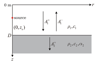
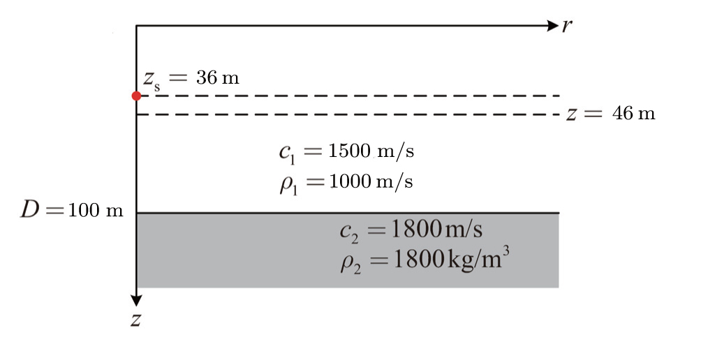
Consider the problem of sound propagation excited by a point source of strength Sω in a Pekeris waveguide involving a homogeneous water column of depth D, sound speed c1, and density ρ1, overlying a homogeneous fluid halfspace of sound speed c2, density ρ2, and attenuation α2. A schematic of this problem is shown in Fig.


 | Fig. 1. Schematic diagram of the Pekeris-waveguide problem. The amplitudes of the down- and upgoing waves in water and that of the downgoing wave in the bottom in the homogeneous solution to the depth-dependent wave equation are denoted by    |
The depth-dependent Green’s function, Ψ(kr,z), can be computed either numerically or analytically. In the subsequent sections we will give these two solutions separately.
Below we first show briefly that the solution to Eq. (
In Ref. [14], the depth-dependent Green’s function in water (0 ≤ z ≤ D) is represented by


By imposing the boundary conditions of vanishing pressure at the sea surface, the continuity of the normal particle displacement at the bottom, and the continuity of pressure at the bottom, we reach the following linear system of equations for the amplitudes of the homogeneous solution to Eq. (

The above linear system of equations is theoretically correct. However, as pointed out in Ref. [5], numerical instability will occur in the evanescent regime kr > k1 when equation (

Noticing the above-mentioned stability problem in Ref. [14], reference [5] gives another system of equations for the amplitudes
In Ref. [5], the depth-dependent Green’s function in water is represented by


As shown above, although both the linear system of equations in Eq. (

By imposing the boundary conditions, we obtain the following linear system of equations

Once the amplitudes
In the previous section we propose an unconditionally stable numerical solution for the amplitudes of the homogeneous solution to the depth-dependent wave equation. As shown below, for the problem of sound propagation in a Pekeris waveguide, we can solve Eq. (
By solving Eq. (


It is obvious that the above analytical solution for the depth-dependent Green’s function in water satisfies reciprocity (the source is assumed to be located in water, as shown in Fig.

Similarly, with ρ2 → ∞, equation (

In addition, with ρ1 = ρ2 and c1 = c2, it can be easily shown that equation (
Once the depth-dependent Green’s function is obtained, the displacement potential, ψ(r,z), can be evaluated by applying the inverse Hankel transform given in Eq. (

As shown in Ref. [5], for a specific wavenumber sampling Δk = (kmax − kmin)/(M − 1), accurate field results can only be obtained up to range R/2, where R is determined by

In this work, the transmission loss for the point-source problem is defined by


Since no approximations have been introduced, the acoustic field thus obtained is exact. Minor accuracy, which is generally negligible, might be sacrificed only in evaluating the wavenumber integral in the inverse Hankel transform.
Normally a point source is appropriate for practical problems in underwater acoustics. However, for purposes such as inter-model comparisons and further extension of a 2D model to a three-dimensional (3D) model, it is also useful to work with a line source in plane geometry.
In this section we consider the problem of sound propagation excited by a line source of strength Sω in a Pekeris waveguide involving a homogeneous water column of depth D, sound speed c1, and density ρ1, overlying a homogeneous fluid halfspace of sound speed c2, density ρ2, and attenuation α2. This problem can also be illustrated schematically by Fig.


By comparing Eq. (

Once the depth-dependent Green’s function is obtained, the displacement potential, ψ(x,z), can be evaluated by applying the inverse Fourier transform given in Eq. (

In this work, the transmission loss for the line-source problem is defined by


It should be pointed out that the expression for the transmission loss used in KRAKEN is different from the exact form as given above and implemented in the present model. The difference arises from the evaluation of the Hankel function. That is, the term 


In this section we consider three numerical examples. The first one involves an ideal waveguide with a pressure-release sea surface and a perfectly reflecting (either pressure-release or rigid) lower boundary. The second one, which involves a Pekeris waveguide, is from Ref. [5], where only field results with a point source are provided. This paper gives both field results with a point source and those with a line source by the present model. The third example also involves a Pekeris waveguide. This example was considered in Ref. [6] to demonstrate how to eliminate the branch cut by the method presented in that paper.
In Section 2 we have shown that the analytical solution for the depth-dependent Green’s function in an ideal waveguide with a pressure-release sea surface and a pressure-release bottom presented in Ref. [5] is wrong. This paper proposes an analytical solution for the depth-dependent Green’s function in a Pekeris waveguide, which reduces to the depth-dependent Green’s function in an ideal waveguide with a pressure-release bottom as ρ2 → 0, and to that in an ideal waveguide with a rigid bottom as ρ2 → ∞. Below we validate our analytical solution through an example. The normal-mode model KRAKEN is used to provide reference solutions.
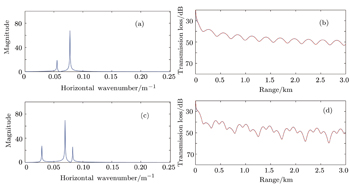
Consider the problem involving an ideal waveguide with a pressure-release sea surface and either a pressure-release or rigid bottom. The water depth is 100 m, and the sound speed and density in water are 1500 m/s and 1000 kg/m3, respectively. A point source is considered, located at depth 36 m and of frequency 20 Hz. The receiver depth is 46 m. For this problem, the convergence criterion given in Eq. (
Figure


 | Fig. 2. Results by the present method and KRAKEN for the ideal waveguide problem. (a) Magnitude of the depth-dependent Green’s function at depth 46 m for the pressure-release bottom case; (b) transmission loss at depth 46 m for the pressure-release bottom case; (c) magnitude of the depth-dependent Green’s function at depth 46 m for the rigid bottom case; (d) transmission loss at depth 46 m for the rigid bottom case. In panels (b) and (d), the blue solid curves correspond to the solutions by the present method, and the red dashed curves correspond to the KRAKEN solutions. |
We now consider another example as schematically shown in Fig.
 | Fig. 3. Pekeris waveguide problem with either a point or a line source. The bottom is either lossless or lossy with an attenuation of 0.5 dB/wavelength. The source frequency is 20 Hz. |
Figure
 | Fig. 4. Magnitude of the depth-dependent Green’s function at a depth of 46 m for the 100-m deep Pekeris waveguide problem with either a lossless bottom (the blue solid line) or a lossy bottom with an attenuation of 0.5 dB/wavelength (the red dashed line). The bottom wavenumber is indicated by the green dashed line. |
Results of transmission loss computed by the present method for this example with a point source and those with a line source are shown in Figs.

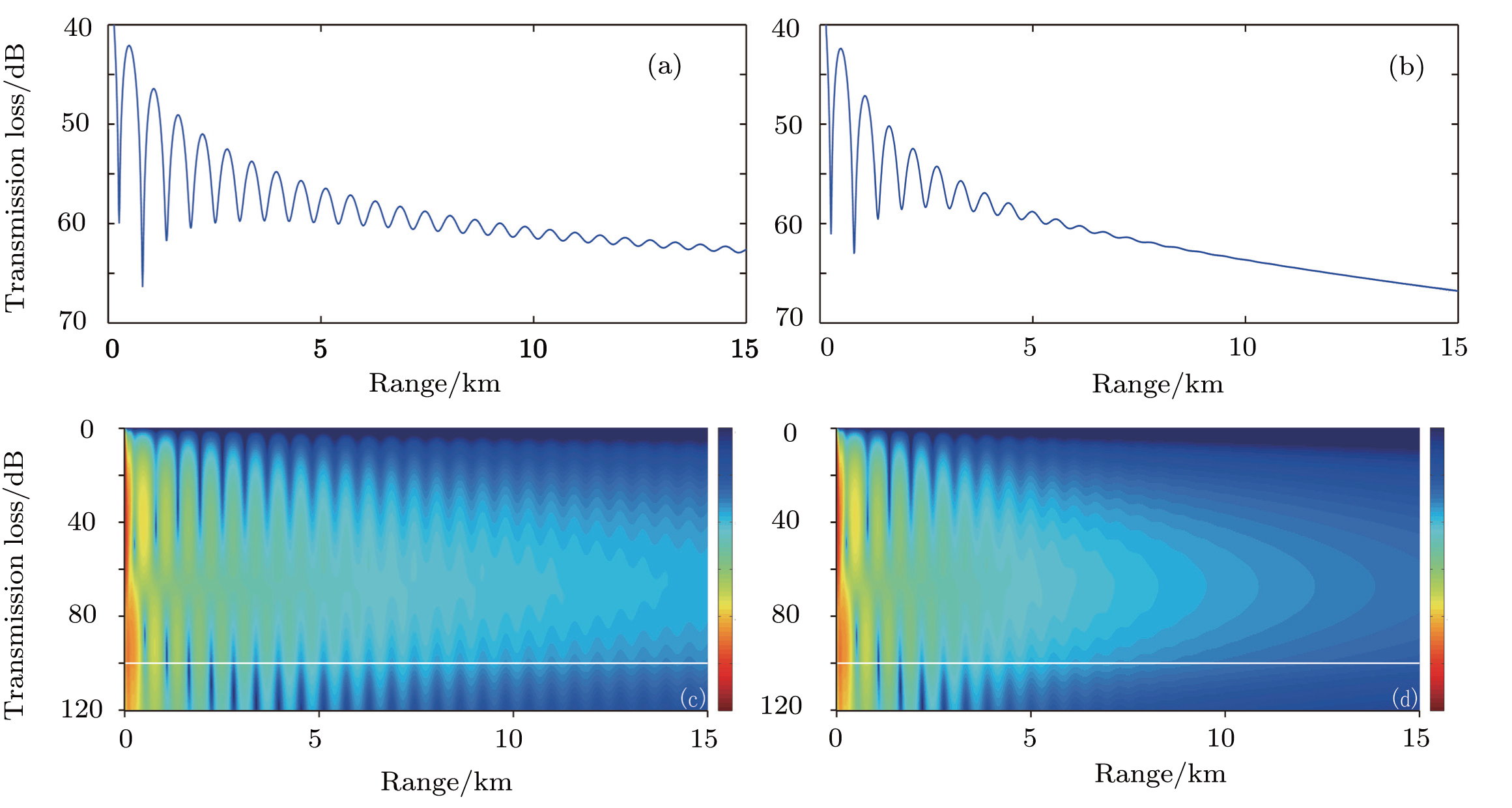 | Fig. 5. Results of transmission loss computed by the present method for the 100-m deep Pekeris waveguide problem with a point source. (a) Transmission loss at a depth of 46 m with a lossless bottom; (b) transmission loss at a depth of 46 m with a lossy bottom with an attenuation of 0.5 dB/wavelength; (c) transmission loss versus range and depth with a lossless bottom; (d) transmission loss versus range and depth with a lossy bottom with an attenuation of 0.5 dB/wavelength. The water-bottom interface is indicated by a white line in panels (c) and (d). |
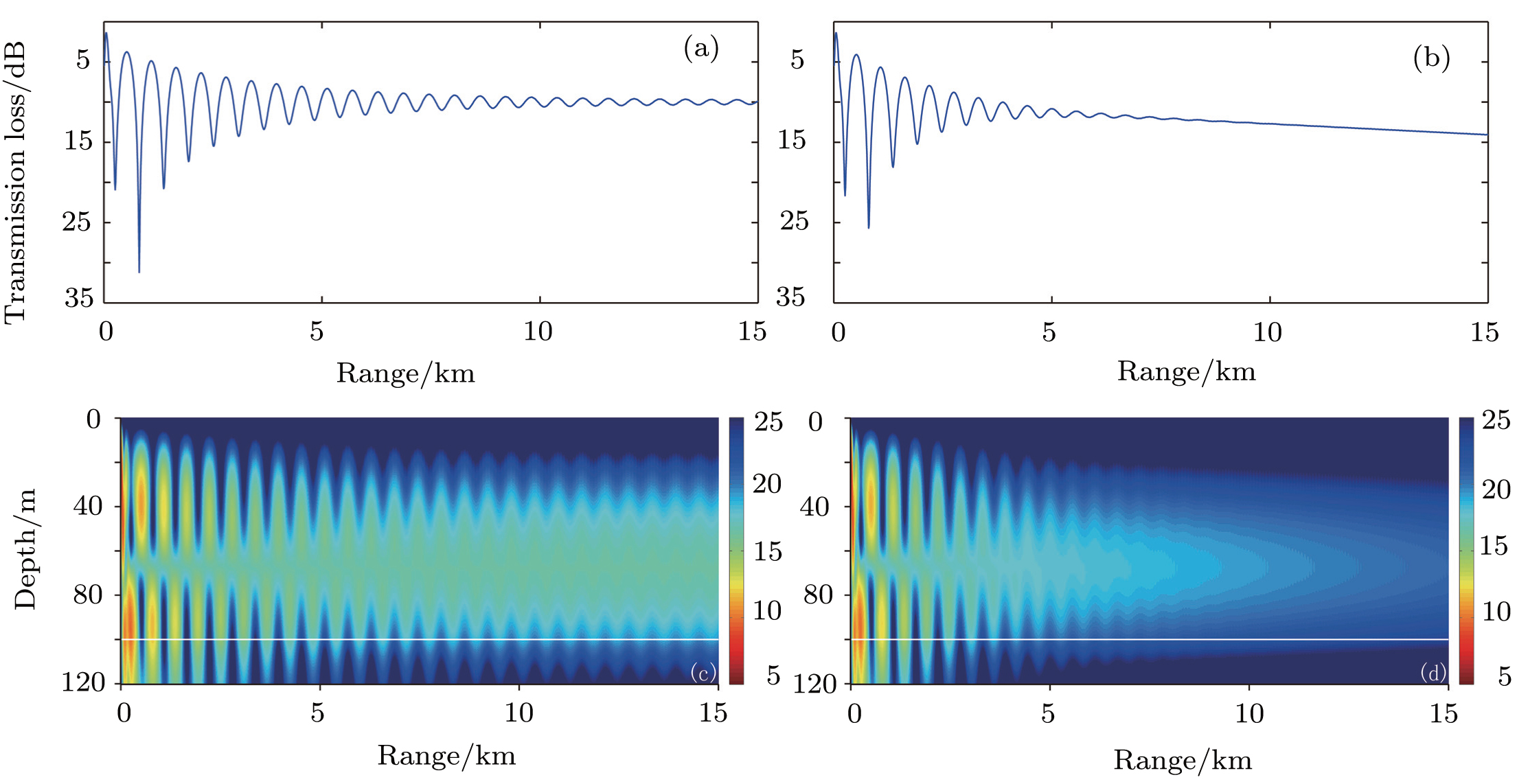 | Fig. 6. Results of transmission loss computed by the present method for the 100-m deep Pekeris waveguide problem with a line source. (a) Transmission loss at a depth of 46 m with a lossless bottom; (b) transmission loss at a depth of 46 m with a lossy bottom with an attenuation of 0.5 dB/wavelength; (c) transmission loss versus range and depth with a lossless bottom; (d) transmission loss versus range and depth with a lossy bottom with an attenuation of 0.5 dB/wavelength. The water-bottom interface is indicated by a white line in panels (c) and (d). |
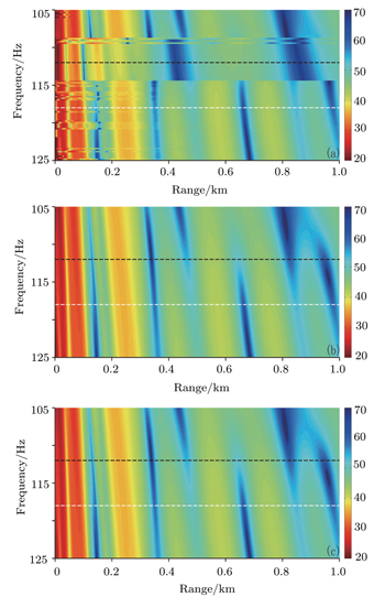
This example involves a lossless Pekeris waveguide with a water depth of 40 m. The source and receiver depths are 20 m and 40 m, respectively. The sound speed and density in water are 1500 m/s and 1000 kg/m3, respectively, and in the bottom they are 1650 m/s and 1500 kg/m3, respectively.
This example was considered in Ref. [6], which shows that at the frequencies where a mode lies near the branch cut, the branch line contribution can be significant at all ranges. Because branch line integrals are cumbersome to compute, and usually their contribution to the total field is significant only in the near field, they are generally neglected in traditional normal mode models. As a result, traditional normal mode models yield inaccurate field solutions at such frequencies. Reference [6] proposed a method to eliminate the branch cuts from the normal mode solution by inserting small attenuation and sound-speed gradients in the lower halfspace. An alternative solution to this problem is to introduce an artificial pressure-release lower boundary at an appropriate depth. For example, the coupled-mode model COUPLE[10,16] introduces an artificial pressure-release lower boundary together with an absorption layer right above this boundary, and applies the Galerkin method to compute the modal solutions. The model DGMCM[11,17] adopts the same method to compute the local modes and is used in this work to provide reference solutions. Below we will analyze this problem and give comparisons of the acoustic field between some of the above-mentioned methods.
Here we give the key parameters for the present model and DGMCM for this problem. For the present model, the convergence criterion given in Eq. (
Figure
 | Fig. 7. Transmission loss versus range and frequency by (a) KRAKEN with a homogeneous halfspace, (b) DGMCM with an artificial pressure-release lower boundary, and (c) the present method. The frequencies 112 Hz and 118 Hz are indicated by the black and white dashed lines, respectively. |
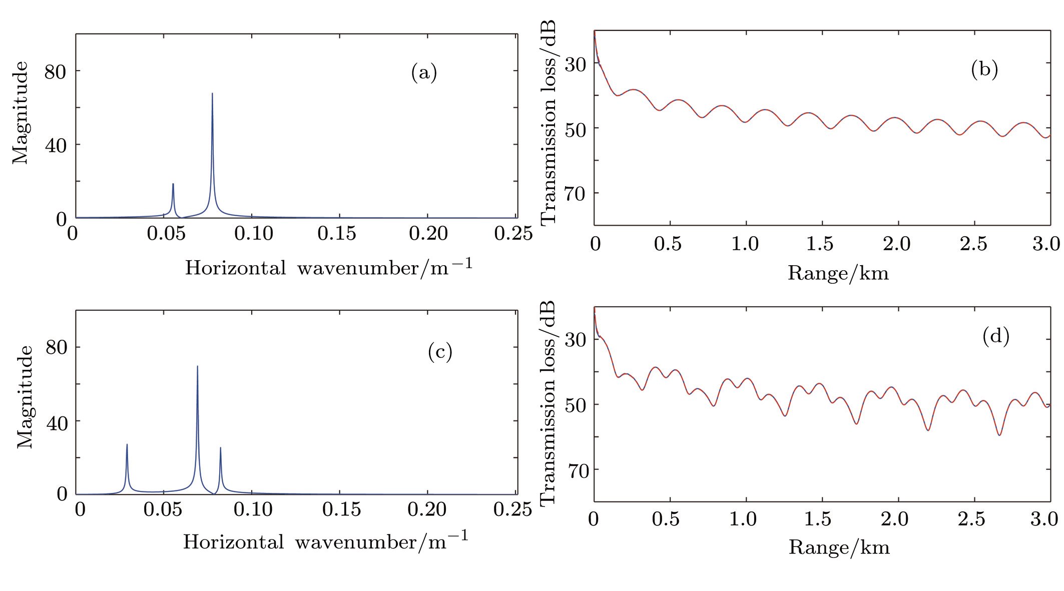
The depth-dependent Green’s functions at a depth of 40 m by the present method at frequencies 112 Hz and 118 Hz are shown in Figs.
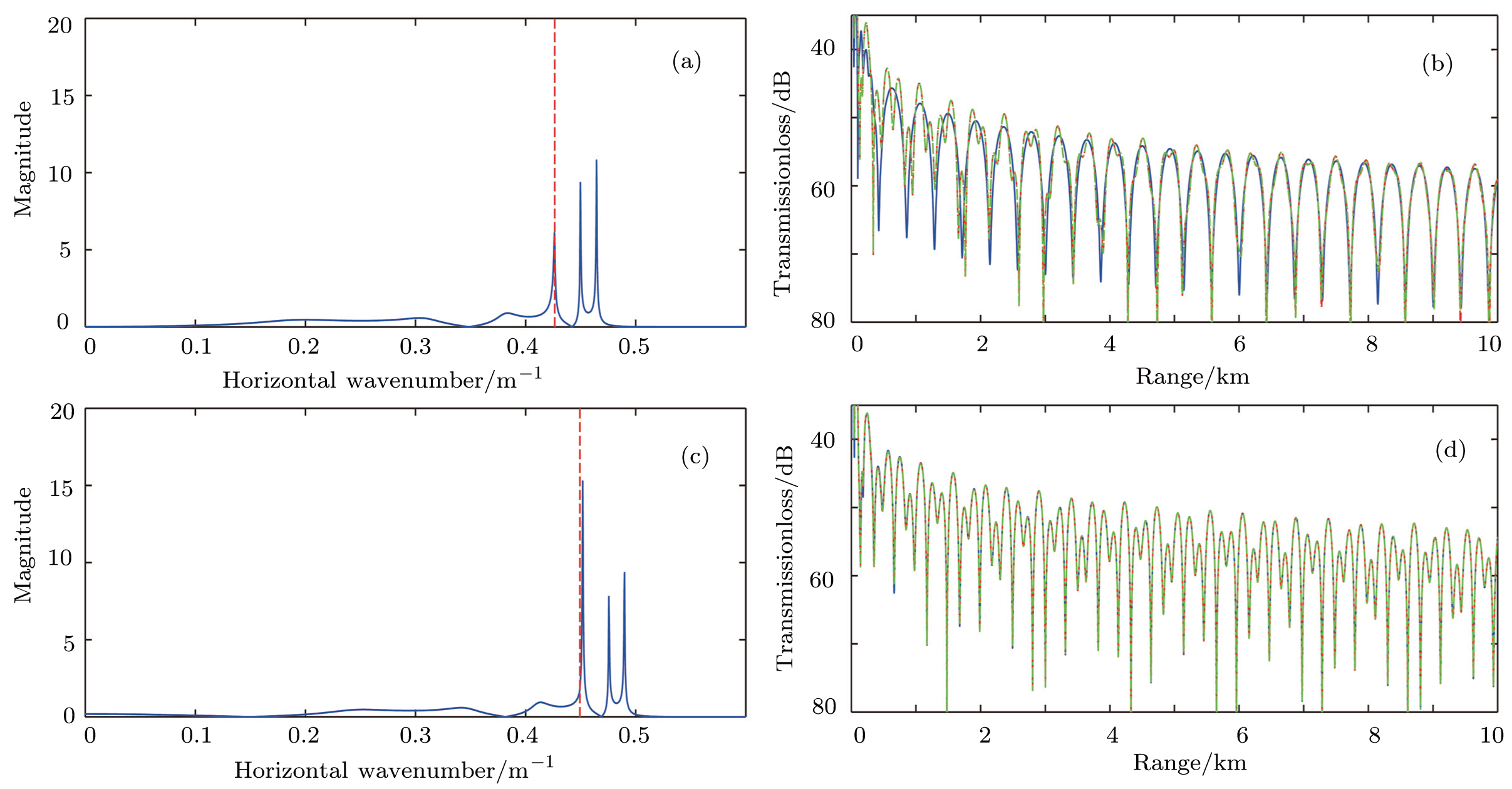 | Fig. 8. (a) Magnitude of the depth-dependent Green’s function at a depth of 40 m at 112 Hz; (b) transmission loss at a depth of 40 m at 112 Hz; (c) magnitude of the depth-dependent Green’s function at a depth of 40 m at 118 Hz; (d) transmission loss at a depth of 40 m at 118 Hz. In panels (a) and (c), the red dashed lines indicate bottom wavenumbers. In panels (b) and (d), the blue solid curves, the red dashed curves, and the green dash-dotted curves are results by KRAKEN with an homogeneous halfspace, DGMCM with an artificial pressure-release lower boundary, and the present method, respectively. |
| Table 1. Horizontal wavenumbers of the first five modes computed by KRAKEN. . |
Finally, we illustrate the convergence criterion regarding wavenumber sampling, M, for the present method through this example with a line source at 118 Hz. At this frequency, from the criterion given in Eq. (
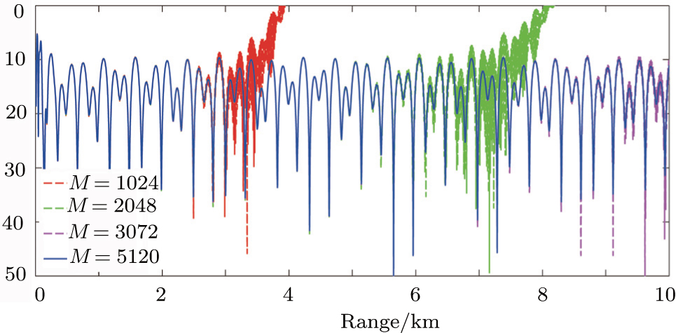 | Fig. 9. Illustration of the convergence criterion regarding the number of sampling points. |
| Table 2. Number of sampling points and corresponding maximum range with accurate field results. . |
An unconditionally stable method based on the wavenumber integration method is first presented for the acoustic field in a Pekeris waveguide. The unconditional stability is achieved by normalizing both the up- and downgoing waves in water and the downgoing waves in the bottom appropriately. Hence, the present numerical solution entirely resolves the stability problem inherent in certain existing methods.
This paper then proposes a closed-form expression for the depth-dependent Green’s function for the Pekeris waveguide problem. It is also illustrated that as the density of the bottom goes to zero, the present analytical solution reduces to that in the ideal waveguide with a pressure-release sea surface and a pressure-release lower boundary; as the density of the bottom goes to infinity, the present analytical solution reduces to that in an ideal waveguide with a pressure-release sea surface and a rigid bottom; and as the density and sound speed of the bottom are separately equal to those in water, the present analytical solution reduces to that in a halfspace. The analytical solution for the depth-dependent Green’s function in a Pekeris waveguide is also implemented in a numerical model, which can deal with the Pekeris waveguide problem with either a point source in cylindrical geometry or a line source in plane geometry.
The wavenumber integration method is well-suited for the problem of sound propagation in shallow water at low frequencies. The present model, which uses the proposed exact solution for the depth-dependent Green’s function, is applied to several numerical examples. Numerical results indicate that the present model can provide accurate field results for general Pekeris problems. However, in the special case where a mode lies very close to the branch cut, KRAKEN might fail to provide accurate field results due to the neglect of the branch line integral. By introducing an artificial pressure-release lower boundary and using the Galerkin method, DGMCM (and COUPLE) can also provide accurate field results, which are in excellent agreement with those by the present model. For a single-frequency calculation, the probability of the occurrence of a mode lying near the branch cut is not great. For broadband calculations, however, the probability is high, as is illustrated in example 3 in this paper. Another scenario with a high probability encountering this phenomenon for single-frequency problems is when the bathymetry varies with range. The coupled-mode models COUPLE and DGMCM can handle this kind of range-dependent problem. However, this is achieved at the cost of having to involve much more normal modes than necessary due to the introduction of an artificial pressure-release lower boundary. We are interested in extending the wavenumber integration method to deal with range-dependent problems, and the present work provides a solid foundation for this research.
In conclusion, since no approximations have been introduced, the present model, which involves an analytical solution for the depth-dependent Green’s function, can provide exact field results and hence serve as a benchmark model for the acoustic field excited by either a point source or a line source in a Pekeris waveguide. Minor accuracy, which is generally negligible, might be sacrificed only in evaluating the wavenumber integral in the inverse Hankel transform.
| 1 | |
| 2 | |
| 3 | |
| 4 | |
| 5 | |
| 6 | |
| 7 | |
| 8 | |
| 9 | |
| 10 | |
| 11 | |
| 12 | |
| 13 | |
| 14 | |
| 15 | |
| 16 | |
| 17 |