


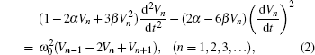
Soliton excitation in the pass band of the transmission line based on modulation
[Zhao Guoying1, Tao Feng2, Chen Weizhong3, †,  ]
]
]
|
|


† Corresponding author. E-mail:
Project supported by the National Natural Science Foundation of China (Grant Nos. 11174145 and 11334005) and the Research Foundation for Young Scientists of Anhui University of Technology (Grant No. QZ201318).
We numerically investigate the excitation of soliton waves in the nonlinear electrical transmission line formed by many cells. When the periodic driving voltage with frequency in the pass band closing to the cutoff frequency is applied to the endpoint of the whole line, the soliton wave can be generated. The numerical results show that the soliton wave generation mainly depends on the self modulation associated with the nonlinear effect. In this study, the lower subharmonic component is also observed in the frequency spectrum. To further understand this phenomenon, we study the dependence of the subharmonic power spectrum and frequency on the forcing amplitude and frequency numerically, and find that the subharmonic frequency increases with the gradual growth of the driving amplitude.
As is well known, in the past few decades, the nonlinear phenomenon has received a great amount of attention. In particular, the soliton has aroused considerable interest ever since its introduction by Benzi et al. in 1981.[1] The soliton can be viewed as representing a balance between the effect of nonlinearity and that of dispersion.[2] In other words, this phenomenon can be found to result from the dynamic interaction between nonlinearity and dissipation. In Ref. [3], the generation of a hole soliton was discussed. Based on the nonlinear Schrödinger equation, the envelope and hole solitons have been also studied well.[4] In recent years, the gap soliton has been progressively reported in a broad variety of nonlinear systems which have periodic structures.[5–9] By means of nonlinear supratransmission,[10,11] Geniet and Leon have investigated the local structure inside the forbidden band, and have given the concept of the cutoff soliton. In addition, the interaction between two solitary waves has been studied in Hertzian chains,[12] and a family of exact solutions describing discrete solitary waves have been presented[13] in a nonintegrable Fermi–Pasta–Ulam (FPU) chain. By using the electromagnetically induced transparency effect which produced high dispersion and nonlinearity, Du et al. have investigated the formation environment and the evolution of the dark soliton with environment parameters.[14] For cases below and above the critical value, bright and dark soliton states admitted by the magnon density distribution have been studied respectively, and the two-soliton collision properties that are modulated by the current have also been discussed.[15] As one of the nonlinear phenomena, the modulational instability has been investigated.[16,17] It can be viewed as the interaction between the nonlinear effect and the dispersive effect. In Ref. [16], the envelope soliton can be induced by the modulational instability that leads to a self induced modulation.
The nonlinear phenomenon has been studied in diverse fields, such as nonlinear optics, fluid dynamics, plasma physics, and the electrical transmission line. Indeed, as a convenient tool, the nonlinear LC transmission line (LCTL), which has N cells consisting of inductors L and nonlinear capacitors C, plays a key role in the research of nonlinear wave propagation. Since the pioneering work by Hirota and Suzuki[18] on a simulation line of the Toda lattice,[19] it has received a great amount of attention in the nonlinear excitation behaviour investigations. In particular, it provides a useful way to study how the wave propagates in a nonlinear dispersive medium and to model the exotic properties of other new systems.[2,20,21] For example, the transmission line can be reduced to the nonlinear Schrödinger model.[22] As the Frenkel–Kontorova and the FPU models are used to investigate the thermal asymmetric energy flux,[23–29] the LCTLs have been used for modulation instability and the gap soliton,[7,9,16,22] and great progress has been achieved.
In view of the soliton investigation with the driving frequency above the cutoff, quite a natural question then arises whether the soliton wave would still occur when the driving frequency is chosen in the pass-band. Indeed, while the linear wave is propagating in the system, the modulational instability would be generated by the nonlinearity and dispersion, and then the self modulation (SM) would be induced. In an optical system, the SM and the soliton excitation have been studied.[30] In this paper, we will choose the appropriate driving amplitude and frequency, and numerically investigate this interesting phenomenon in the LCTL. The outline of the paper is as follows. In Section 2, we will present the model first, which is, in fact, a nonlinear LCTL consisting of many identical cells. In Section 3, we numerically investigate the soliton excitation on the nonlinear electrical network. The dependence of the subharmonic power spectrum and frequency on forcing parameters will be discussed in Section 4. Finally, Section 5 is devoted to some concluding remarks.
The system under consideration is a lossless nonlinear discrete LCTL which is comprised of many elementary cells as shown in Fig.

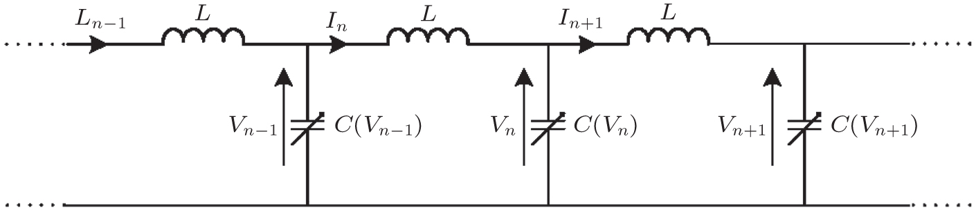 | Fig. 1. Schematic representation of the lossless LCTL where each cell consists of a linear inductor L and a nonlinear capacitor C(V), and all cells have the same structure and parameters. The In and Vn denote the current flowing through the inductor and the reverse voltage applied to the capacitor, respectively. |
Applying the Kirchhoff’s laws and the capacitance–voltage relationship represented by Eq. (


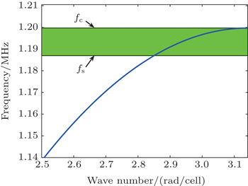
 | Fig. 2. Linear dispersion curve of the LCTL. The driving frequency is chosen in the (green) shade area which satisfies the relation P(ω) × Q(ω) > 0 with P(ω) and Q(ω) being the dispersion coefficient and the nonlinear coefficient, respectively. fc and fs are the upper and lower boundary frequencies of the (green) shade domain (fc is also the cutoff frequency of system). |
In the study, in order to generate the soliton wave, the fs is the lower frequency which can be chosen by the driving one, and the magnitude of fs is 1.0403 MHz. Namely, the driving frequency satisfies

In Refs. [16] and [22], the dispersion curve (see Fig.

In the whole area, the P(ω) is always negative, whereas the Q(ω) can be positive or negative, depending on the carrier wave frequency ω. In our study, the green region selected in Fig.
In fact, in the study, the LCTL has the length N which is long enough to avoid the free end reflections, so that the soliton wave can well keep its propagation. Of course, the wave propagation of the internal cells still obeys Eq. (

In this section, in order to generate the soliton wave, we perform the numerical simulations on the LCTL [Eq. (
The values of L, C0, α, and β have been given in Section 2. The frequency and amplitude of the driving voltage are f = 1.1990 MHz and A0 = 0.3 V, respectively. Obviously, the driving frequency value is located in the pass band (see the green area in Fig.
Figure
 | Fig. 3. Final state of the LCTL at the end of simulation for a driving frequency f = 1.1990 MHz and amplitude A0 = 0.3 V. The (red) horizontal line denotes the driving amplitude value A0. |
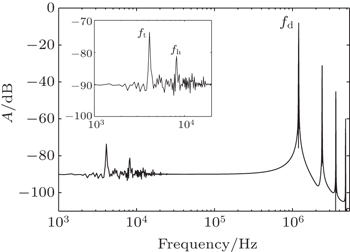
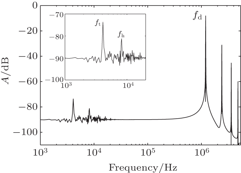
Here, we also calculate the frequency spectrum of a 100-th cell wave by using the fast Fourier transform algorithm (FFT) as shown in Fig.
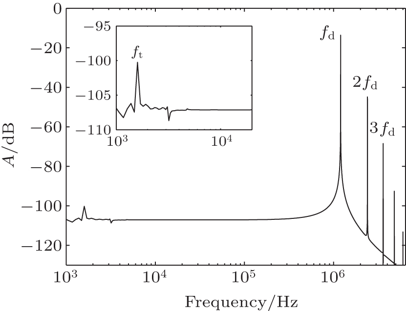 | Fig. 4. Plot of frequency spectrum versus frequency of the 100-th cell wave. The fd represents the driving frequency, and the ft denotes the subharmonic frequency. The inset shows the magnified portion in the lower frequency range from 1 kHz to 20 kHz. The calculating conditions are f = 1.1990 MHz and A0 = 0.30 V. |
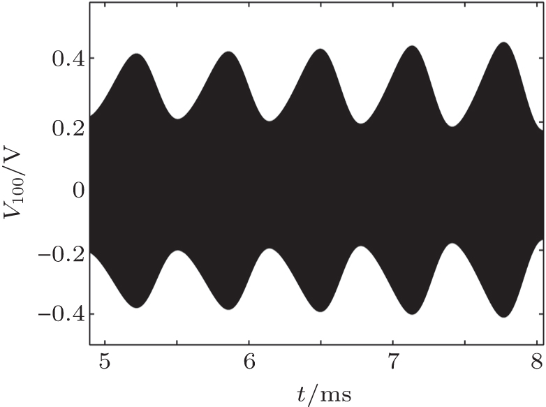 | Fig. 5. Time response of the 100-th cell. The driving frequency and amplitude are f = 1.1990 MHz and A0 = 0.30 V, respectively. |
 | Fig. 6. The FFT power spectrum calculated at the 100-th cell. The driving frequency and amplitude are f = 1.1990 MHz and A0 = 0.60 V, respectively. The fd represents the fundamental frequency, while the ft and fh denote the subharmonic frequencies. |
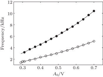
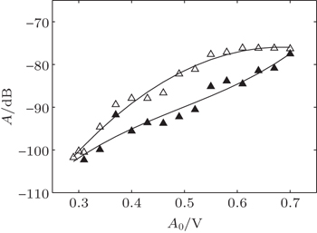
In this section, we turn our attention to the dependence of SH on the driving parameters f and A0. By investigation, the modulation is found to vary with f and A0. That is to say, the modulation will become strong with the driving frequency f or (and) amplitude A0 increasing. In the spectrum, we can also clearly find the SH component. As a result of the process of the f or/and A0 increasing, there emerges a second SH fh coexisting with the first one ft. Meanwhile, the SH frequency and power would change correspondingly.
Figure
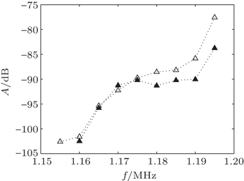
 | Fig. 7. Plots of subharmonic frequency versus the driving amplitude A0 at the fixed driving frequency 1.1990 MHz. The empty and solid circles represent the frequencies for ft and fh, respectively. |
The variations of SH amplitude A with driving amplitude A0 are calculated and shown in Fig.
 | Fig. 8. Plots of subharmonic amplitude A versus driving amplitude A0 at the fixed driving frequency 1.1990 MHz. The empty and solid triangles represent the amplitudes for ft and fh, respectively. |
Figure
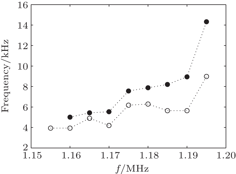 | Fig. 9. Variations of subharmonic frequency with driving frequency f at the fixed driving amplitude 0.7 V. The empty and solid circles represent the amplitudes for ft and fh, respectively. |
The relation between subharmonic amplitude A and the driving frequency f is plotted in Fig.
 | Fig. 10. The relation between the subharmonic amplitude A and the driving frequency f at a fixed driving amplitude of 0.7 V. The empty and filled triangles represent the amplitudes for ft and fh, respectively. |
From the above, it is easy to understand the soliton wave generation in the LCTL if we consider the nonlinear and modulation effect. Obviously, from Eq. (
We know that the higher the driving amplitude, the stronger the nonlinear effect is. When the linear wave propagates in the LCTL, the result is that the modulation is induced by the nonlinearity. The numerical data illustrate that the modulation would be enhanced by increasing the driving frequency or/and amplitude. The subharmonic components are closely related to both the driving frequency and the driving amplitude. In the system, the nonlinear effect leads to the generation of subharmonics. From the spectrum, the simulation results show that the subharmonic amplitude is dependent on the driving amplitude A0. It indicates that the amplitude of the subharmonic will increase with an increase in the nonlinear effect.
In this work, we numerically investigate the generation of soliton waves in the simple LCTL consisting of many cells, and all the cells have the same structure and the same parameters. We can clearly see that the soliton wave can be generated in the pass band based on the SM. When the driving wave propagates in the LCTL, the SM will be induced by the nonlinear effect. This mechanism of the soliton wave generation is completely different from the one which depends on the supratransmission in the forbidden band.[22,29] As a matter of fact, the choosing of the driving frequency is very important for the soliton wave generation. While the driving frequency is located in the special region of the linear dispersion curve (see the green area of Fig.
| 1 | |
| 2 | |
| 3 | |
| 4 | |
| 5 | |
| 6 | |
| 7 | |
| 8 | |
| 9 | |
| 10 | |
| 11 | |
| 12 | |
| 13 | |
| 14 | |
| 15 | |
| 16 | |
| 17 | |
| 18 | |
| 19 | |
| 20 | |
| 21 | |
| 22 | |
| 23 | |
| 24 | |
| 25 | |
| 26 | |
| 27 | |
| 28 | |
| 29 | |
| 30 |