

Compressed sensing sparse reconstruction for coherent field imaging
[Cao Bei†,  , Luo Xiu-Juan, Zhang Yu, Liu Hui, Chen Ming-Lai]
, Luo Xiu-Juan, Zhang Yu, Liu Hui, Chen Ming-Lai]
|
|


† Corresponding author. E-mail:
Project supported by the National Natural Science Foundation of China (Grant No. 61505248) and the Fund from Chinese Academy of Sciences, the Light of “Western” Talent Cultivation Plan “Dr. Western Fund Project” (Grant No. Y429621213).
Return signal processing and reconstruction plays a pivotal role in coherent field imaging, having a significant influence on the quality of the reconstructed image. To reduce the required samples and accelerate the sampling process, we propose a genuine sparse reconstruction scheme based on compressed sensing theory. By analyzing the sparsity of the received signal in the Fourier spectrum domain, we accomplish an effective random projection and then reconstruct the return signal from as little as 10% of traditional samples, finally acquiring the target image precisely. The results of the numerical simulations and practical experiments verify the correctness of the proposed method, providing an efficient processing approach for imaging fast-moving targets in the future.
Coherent field imaging, also referred to as a Fourier telescope (FT), is a novel and promising active imaging technique, having the potential to achieve high resolution images for satellite targets as far as geosynchronous target ranges.[1,2] In contrast to traditional imaging techniques, coherent field imaging is capable of imaging the targets through atmospheric turbulence, and the imaging quality is immune to downlink the turbulence effect[3,4] and optical quality of the receiver. It has therefore drawn considerable attention in recent years, becoming a promising candidate in the field of space surveillance and object recognition.[5,6]
Based on the computational imaging principle, coherent field imaging can produce good images from the target spatial frequency components encoded in the temporal signal reflected from the target, therefore return signal processing and reconstruction is essentially significant in the whole imaging system. By fine recovery and reconstruction of the return signal, the target image can be obtained with high resolution. At present, researchers have introduced some feasible approaches to improve the performance of return signal processing.[7,8] However, these methods are generally based on a requirement for sampling all the complete information about the return signal in data acquisition. If the inherent characteristic of the signal itself is considered, a more efficient processing scheme can be obtained.
Compressed sensing (CS) is a novel mathematical theory for sampling and reconstructing signals in an efficient way.[9] The CS has been previously reported in single-pixel imaging,[10] radar imaging,[11] and inline single-shot holography for tridimensional imaging.[12]
According to the analysis of sparsity for the return signal, we propose a genuine CS-based sparse reconstruction (CS-SR) scheme for coherent field imaging. Firstly, the sparse factor of the received signal is determined, then an effective random projection is implemented to greatly reduce the number of samples required in data acquisition, hence recovering the return signal from as little as 10% of random measurements, finally achieving the reconstructed image with high precision. The simulations and practical experiments prove the validity of CS-SR, developing an efficient processing approach for coherent field imaging in the applications of imaging fast-moving targets.
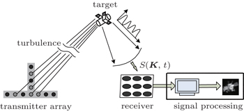
Coherent field imaging is an active imaging technique based on computational imaging theory, which uses multiple beams from spatially separated transmitters to illuminate a distant target. Based on the spatial-temporal coding principle, the target spatial frequency components are encoded in the temporal signal reflected from the target. By collecting the return signal in the receiver and eliminating random atmospheric phase errors in the uplink turbulence by phase closure, the true amplitude and phase of the target can be recovered and processed to reconstruct the target image. The schematic diagram of the imaging principle is shown in the following figure (Fig.
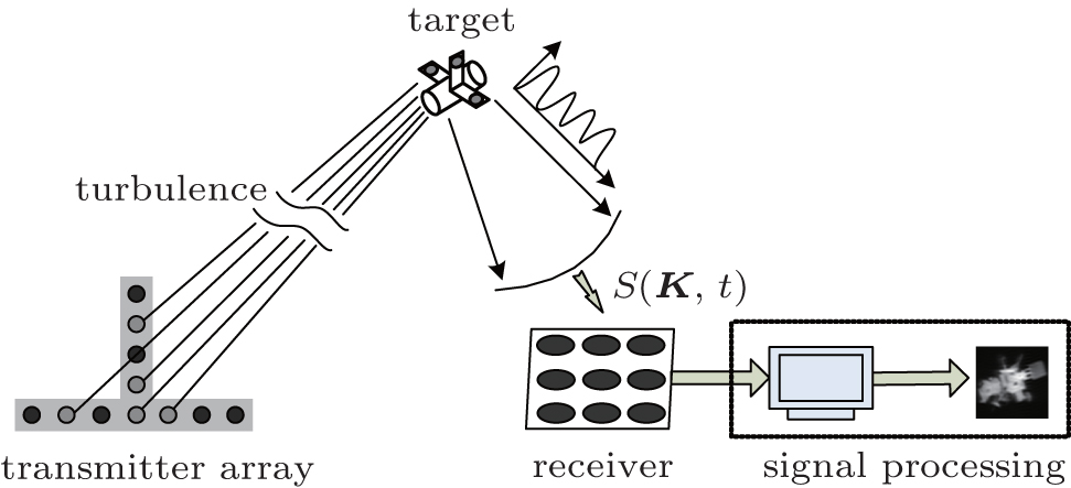 | Fig. 1. Schematic diagram of coherent field imaging. |
The return signal S(

The traditional return signal processing is realized under the constraint of the Nyquist sampling theorem. All the complete information about the received signal needs to be sampled for extracting the important spectrum information providing for the next image reconstruction. However, in the applications for imaging fast-moving objects, the imaging time is a crucial issue. It will be favorable to accelerate the processing efficiency of data acquisition. From this angle, we are to explore a novel and efficient processing scheme to provide a better solution.
Based on the imaging principle of coherent field imaging, if the return signal is sparse and compressible, it is possible to realize a more efficient way in the process of signal processing. CS is a novel signal processing theory that allows data reconstruction with fewer samples than traditionally required. As long as the original signal is sparse in some basis, it is possible to recover N pieces of information in object space from M ≪ N incoherent measurements with high confidence.
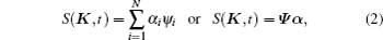
We firstly analyze the characteristic of the return signal. By illuminating a target with a fringe pattern that sweeps across it due to frequency differences between laser beams, the received signal in the time domain is a linear combination of several cosine signals. Therefore we transform the return signal into the Fourier spectrum domain to reveal that it is sparse and satisfies the precondition for applying CS. Fourier transform is used as a sparse basis matrix, then an N × 1 original return signal S(

According to the condition that the received signal is compressible, instead of sampling the entire data, we perform a compressed data acquisition under CS theory and put forward a novel CS-SR scheme for signal processing in coherent field imaging. The realization of CS-SR includes two steps: random projection and sparse reconstruction.
The measurement process is formulated as


We select
By the above random projection process, the number of the return signal samples can be greatly reduced from
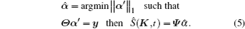
The reconstruction error is defined as the form: e = norm(Ŝ − S)/norm(S), where S is the original return signal, Ŝ represents the reconstructed signal, and norm(×) denotes the norm operation. The error e can be reduced by properly choosing M and iteration times of the reconstruction process.
At the end, based on the reconstructed return signal, a robust all-phase FFT target reconstruction algorithm[15] is used to reconstruct the target image. The realization chart is shown in Fig.
 | Fig. 2. Realization chart of CS-SR scheme. |
In this section, we present both the numerical simulations and the practical measurements to verify the validity of the CS-SR scheme by comparison with the traditional reconstruction (TR) scheme.
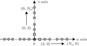
The basic parameters of the coherent field imaging system are set as follows: the wavelength of the laser is 1064 nm, the imaging distance is 60 m, the target size is 4 mm; the T-type transmitter array is adopted and three beams are transmitted simultaneously at the same moment. The demonstration of the baseline location is shown in Fig.
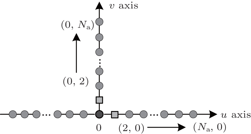 | Fig. 3. Demonstration of baseline configuration in T-type array. |
We numerically simulate the intensity accumulation of the return signal at the object plane by receiving and processing the return signal to reconstruct the target image. In the simulations, the modulated frequencies among three beams are chosen to be [0,1,3] × 10 kHz, and the sampling rate is 1 MHz, sampling 500 samples in each baseline location.
Firstly, we verify the signal reconstruction precision of CS-SR in an ideal environment. The signal-to-noise (SNR) level is set to be 200 dB. In the CS-SR scheme, the dimension of random measurements should satisfy M ≥ 22, which is a least requirement under the condition of sparse factor K = 3. We set M = 23 and M = 44 to separately reconstruct the return signal, and iteration times are set to be 4, i.e., 4 times sparse factor. The reconstruction error in the u axis sampling is computed and listed in Table
| Table 1. Reconstruction errors of CS-SR in u-axis sampling (Na = 8). . |
As Table
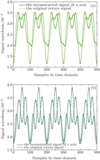
Figure
 | Fig. 4. Reconstructed return signals of CS-SR: (a) u axis data sampling; (b) v axis data sampling. |
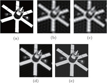
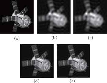
According to the reconstructed return signal by CS-SR, we reconstruct the target image by all-phase FFT reconstruction and compare the results with those of TR. Figure
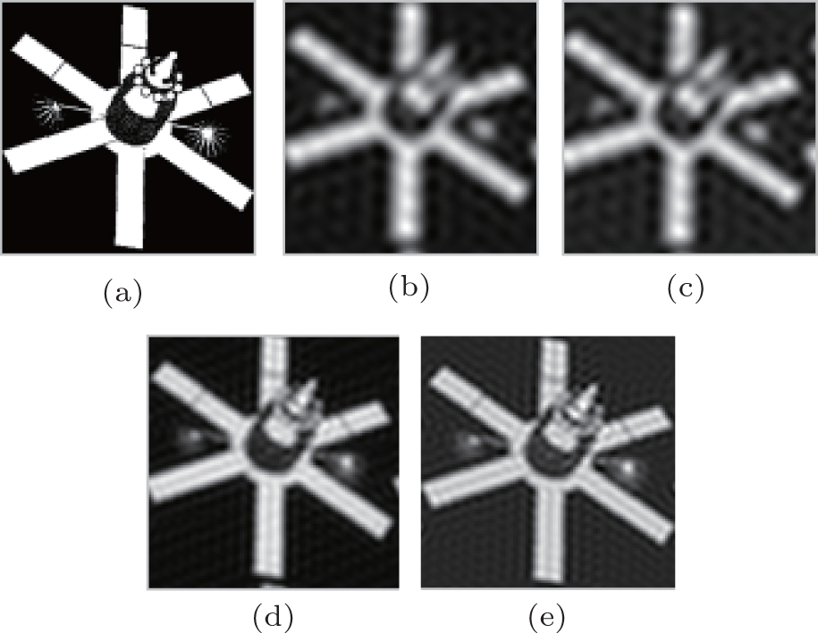 | Fig. 5. Comparison among the reconstructed images: (a) simulated target 1; (b) the reconstructed image by TR (Na = 10); (c) the reconstructed image by CS-SR (Na = 10); (d) the reconstructed image by TR (Na = 20); (e) the reconstructed image by CS-SR (Na = 20). |
As figure
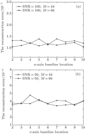
To test the reconstruction performance of CS-SR in a noise environment, we add white Gaussian noise to the simulated return signal and set different SNR levels. Referring to the situation of an ideal environment, we set the random measurements of CS-SR, i.e., M = 44 and M = 66. The reconstruction errors of u-axis sampling and v-axis sampling at each baseline location are shown in Figs.
 | Fig. 6. Reconstruction errors: (a) u-axis sampling; (b) v-axis sampling. |
As shown in Fig.
 | Fig. 7. Comparison among the reconstructed images: (a) simulated target 2; (b) the reconstructed image by TR (Na = 10); (c) the reconstructed image by CS-SR (Na = 10); (d) the reconstructed image by TR (Na = 20); (e) the reconstructed image by CS-SR (Na = 20). |
According to the above results, in order to obtain satisfactory reconstructed quality in a noise environment with low SNR, it is necessary to increase the number of random measurements in the CS-SR scheme. The quantity of the required samples is still much less than TR desires, which indicates that the determination of the sparse factor is a key issue in sparse reconstruction for coherent field imaging. Combined with the correct selection of measurement dimension, CS-SR can achieve good reconstruction performance even in a noisy environment.
The effectiveness of CS-SR is validated by the numerical simulations in Subsection 4.1. Then we apply CS-SR to an outdoor imaging system for the return signal processing and reconstruction.[15] Three different transmissive targets are adopted and a T-type array baseline scale is set to be 15 × 16. The modulated frequencies between three beams are chosen to be 0, 50 kHz, and 150 kHz respectively, and the sampling rate is 4 MHz.
We sample 4000 data points by TR at each baseline location. In terms of the outdoor SNR level, the measurement is in a range of 50 dB–70 dB; we set different values of random measurements in CS-SR and observe the reconstruction errors. According to the basic RIP rule, the dimensions of measurements should satisfy M ≥ 31. Therefore, we first set the initial value of random samples to be M = 62. The random projection measurement is implemented with the Gaussian random matrix by directly projecting the original samples to the measurement space and making sure that no important frequency information is damaged in the projection process. Based on the CS-SR scheme, the mean value ē and standard deviation δ of the reconstruction error are separately computed for each target, and the results are listed in Table
| Table 2. Reconstruction errors computed for three targets. . |
It is revealed from Table
According to experimental data, we set iteration times to be six times sparse factor to ensure a fast convergence in the reconstruction process. Considering the following three kinds of targets, the reconstructed images by TR and CS-SR with M = 500 are shown respectively in Figs.
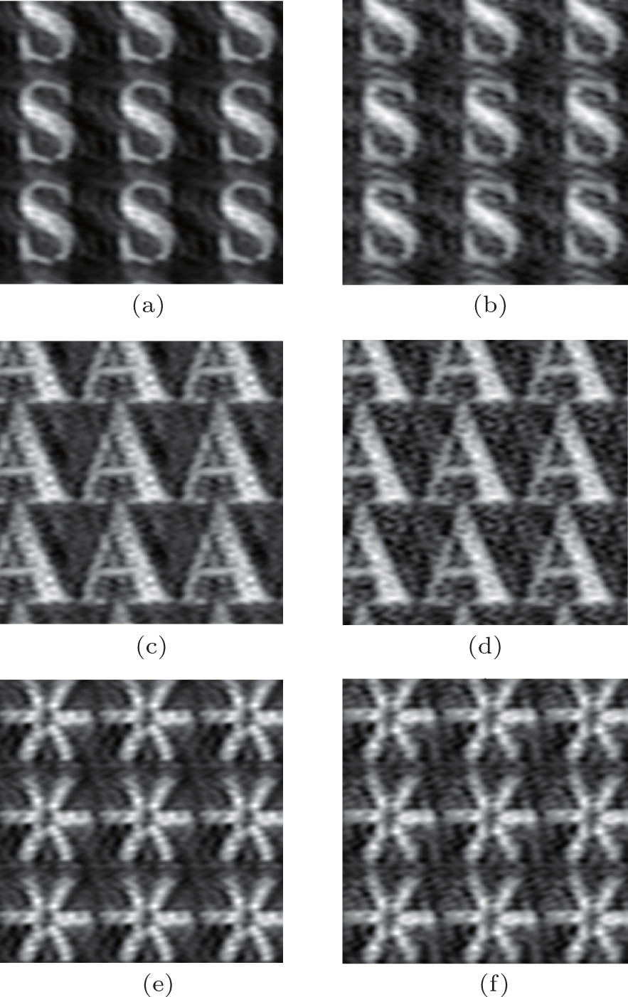 | Fig. 8. Reconstructed images based on experimental data: (a) the reconstructed target S by TR; (b) the reconstructed target S by CS-SR; (c) the reconstructed target A by TR; (d) the reconstructed target A by CS-SR; (e) the reconstructed target six by TR; (f) the reconstructed target six by CS-SR. |
Figure
| Table 3. Image Strehl values of Fig. |
The Strehl values of the reconstructed image by CS-SR are slightly lower than those of TR. For that the precision of signal reconstruction is not so high as that in the simulations considering the existence of noises in a practical outdoor environment. Nevertheless the target is still clearly recognizable. Therefore, the proposed CS-SR scheme provides an efficient means to enhance the sampling efficiency in data acquisition for coherent field imaging.
In this paper, we present a genuine CS-SR scheme for coherent field imaging. Based on the analysis result that the received signal is sparse and compressible, we accomplish effective random projection to greatly reduce the required samples in data acquisition, and finally reconstruct the return signal with high accuracy by much fewer measurements. The effectiveness of the CS-SR scheme is validated by simulations and practical experiments, showing that the CS-SR scheme provides an efficient signal processing approach and promoting the applications of coherent field imaging in fast-moving target imaging.
| 1 | |
| 2 | |
| 3 | |
| 4 | |
| 5 | |
| 6 | |
| 7 | |
| 8 | |
| 9 | |
| 10 | |
| 11 | |
| 12 | |
| 13 | |
| 14 | |
| 15 | |
| 16 |