
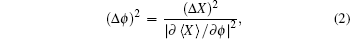
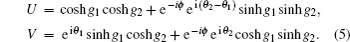
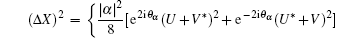
Phase sensitivity of two nonlinear interferometers with inputting entangled coherent states
[Chao-Ping Wei, Hu Xiao-Yu, Yu Ya-Fei, Zhang Zhi-Ming†,  ]
]
]
|
|


† Corresponding author. E-mail:
Project supported by the Major Research Plan of the National Natural Science Foundation of China (Grant No. 91121023), the National Natural Science Foundation of China (Grant Nos. 11574092, 61378012, and 60978009), the Specialized Research Fund for the Doctoral Program of Higher Education of China (Grant No. 20124407110009), the National Basic Research Program of China (Grant Nos. 2011CBA00200 and 2013CB921804), and the Program for Innovative Research Team in University (Grant No. IRT1243).
We investigate the phase sensitivity of the SU(1,1) interfereometer [SU(1,1)I] and the modified Mach–Zehnder interferometer (MMZI) with the entangled coherent states (ECS) as inputs. We consider the ideal case and the situations in which the photon losses are taken into account. We find that, under ideal conditions, the phase sensitivity of both the MMZI and the SU(1,1)I can beat the shot-noise limit (SNL) and approach the Heisenberg limit (HL). In the presence of photon losses, the ECS can beat the coherent and squeezed states as inputs in the SU(1,1)I, and the MMZI is more robust against internal photon losses than the SU(1,1)I.
Phase estimation is one of the most important issues in quantum metrology and has been widely studied.[1] Optical interferometers are the main devices for metrology and weak signal detection.[2] The ultimate goal of phase estimation is to enhance the phase sensitivity of the interferometers and to attain the Heisenberg limit (HL).[3] Theoretically, there are two main ways to enhance the phase sensitivity of interferometers. One way is using some specific quantum states, such as the squeezed states, the superposition and entanglement states to decrease the quantum noise.[4–9] The other way is using the nonlinear effects to increase the phase signal. As is shown in Ref. [10], because of the gain in the optical parametric amplifiers (OPAs), the maximum output intensity of the interferometer can be much bigger than the input intensity as well as the intensity inside the interferometer, and has better sensitivity than the traditional linear interferometer. Therefore, we can enhance the phase sensitivity with the help of the OPA. For example, the phase sensitivity and signal-to-noise ratio of the SU(1,1) interferometer (SU(1,1)I)[11] can be improved greatly due to the gain of the OPAs. Many of these theories for improving the phase sensitivity of interferometers have been confirmed by experiments in recent years.[12,13]
In this paper, we discuss a nonlinear interferometer which is composed of a beam splitter (BS) and an OPA.[14] It can be treated as a variation of the Mach–Zehnder interferometer (MZI) which is composed of two BSs. For simplicity in nomenclature, we name this nonlinear interferometer as the modified Mach–Zehnder interferometer (MMZI). It can also be treated as a variation of the SU(1,1)I which is composed of two OPAs. It is well known that the OPAs not only amplify the signal light but also amplify the noise, so we replace the second OPA in the SU(1,1)I with a BS to balance the signal and noise, and this forms the MMZI. We use the entangled coherent state (ECS)[15] as the input of the interferometer since the ECS can reduce the quantum noise and is robust against photon losses.[16] In real experiments, the photon losses are inevitable and have great effects on the phase sensitivity, therefore, we will also discuss these effects in the MMZI and in the SU(1,1)I.
The organization of this paper is as follows. In Section 2, we propose a special nonlinear optical interferometer in which there is a black box. If the black box is an OPA, then the interferometer is the so-called SU(1,1)I, and if the black box is a BS, then the interferometer is the so-called MMZI. Afterwards we study the phase sensitivity of these two interferometers with the ECS as inputs and make a comparision with the linear MZI. In Section 3 we study the effects of the photon losses on the phase sensitivity of the interferometers, and we also make a comparison with other approaches. Section 4 presents the conclusions.
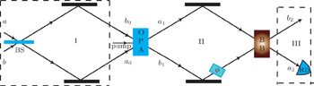
An important problem with the optical interferometers is to improve the phase sensitivity as far as possible. Here, we discuss a special nonlinear interferometer, as shown in Fig. 

 | Fig. 1. A nonlinear optical interferometric setup which is composed of three parts. Part I is for preparing the input states to the main body of the interferometer (Part II), and Part III is for detection. The prepared states from Part I and the pump light go through an OPA. There is a phase shifter in one arm of the interferometer, and the light will carry phase information after passing through it. Before the detection, there is a black box BB, which may be a BS or an OPA, which represents an MMZI or an SU(1,1)I, respectively. The homodyne detection is implemented to the output mode a2. |
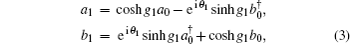
The SU(1,1)I was proposed in Ref [18], and has been studied with different quantum states as inputs in recent years.[19–21] In an SU(1,1)I, the two BSs of a conventional Mach–Zehnder interferometer(MZI) are replaced by two OPAs which are characterized by the SU(1,1) group.[18,22] The OPA is a device that can transfer energy from a strong pump beam to two signal beams, and a detailed description can be found in Ref. [21]. The phase sensitivity of an SU(1,1)I can approach the HL in the condition of no photon losses. Here we use an ECS as the input of the SU(1,1)I. For the first OPA, the relationship between the operators of the output modes (a1, b1) and the input modes (a0, b0) is given by[23]

By using Eqs. (

The MMZI can be obtained when the black box in Fig.

Combining Eqs. (

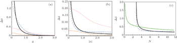
To compare the optimal phase sensitivity of the two interferometers with the shot-noise limit (SNL) 
According to Eqs. (
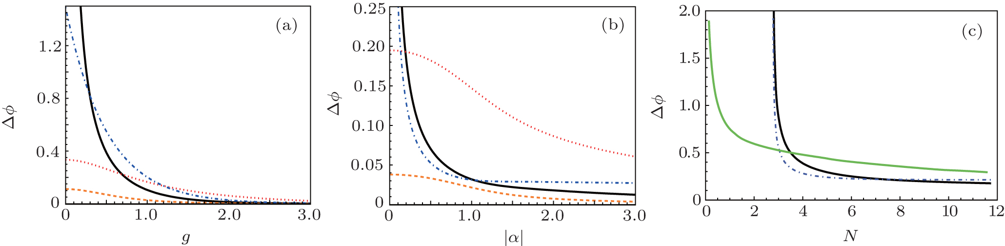 | Fig. 2. (a) The phase sensitivity against the gain factor g for a given |α| = 3, and θα = π/2. (b) The phase sensitivity against the amplitude |α| for a given g = 2 and θα = π/2. (c) The phase sensitivity against the total average photon number N. Black solid line: SU(1,1)I; blue dot-dashed line: MMZI; red dotted line: the shot-noise limit  |
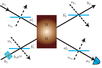
In real experimental environments, the photon losses and detection efficiency have great effects on the precision and phase sensitivity.[25,26] In the presence of photon losses, especially with the internal losses, the phase sensitivity decoheres very quickly because of the amplification of the vacuum noise. For instance, the HL can be approached for the maximally path-entangled N00N state when there is no photon losses, but is very vulnerable under photon losses.[27,28] Therefore, it is necessary to enhance the robustness of interferometers against losses. Here we replace the second OPA of the SU(1,1)I with a BS to balance the signal and noise, and use four fictitious BSs to model photon losses in the two modes (Fig.
 | Fig. 3. (a) The schematic diagram of the photon losses after the phase shifter and before detection. The photon losses are modeled by four fictitious beam splitters. |
For the lossy SU(1,1)I, the relations among the operators in Fig.
By combining Eq. (

For the lossy MMZI, the relations among the operators in Fig. 
Figure
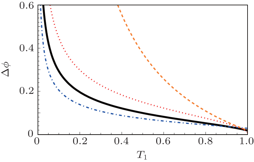 | Fig. 4. The phase sensitivity Δϕ as a function of the internal transmissivity rates T1 with |α| = 3, and θα = π/2. The black solid and blue dot-dashed lines represent the results of Eqs. ( |
In conclusion, we investigated two nonlinear interferometers (MMZI and SU(1,1)I) and discussed their phase sensitivity with the ECS as inputs. We found that the phase sensitivity can beat the SNL and approach the HL for large gain factor g and amplitude |α|, and the two nonlinear interferometers outperform the linear MZI for a larger average photon number in the absence of photon losses. Particularly, the phase sensitivity of the MMZI is more robust to photon losses than that of the SU(1,1)I in a wide region of losses. Both MMZI and SU(1,1)I with ECS inputs can beat the SU(1,1)I with |α〉 |ξ〉 inputs. Nevertheless, the phase sensitivity can still beat the SNL so long as the photon losses are small enough.
| 1 | |
| 2 | |
| 3 | |
| 4 | |
| 5 | |
| 6 | |
| 7 | |
| 8 | |
| 9 | |
| 10 | |
| 11 | |
| 12 | |
| 13 | |
| 14 | |
| 15 | |
| 16 | |
| 17 | |
| 18 | |
| 19 | |
| 20 | |
| 21 | |
| 22 | |
| 23 | |
| 24 | |
| 25 | |
| 26 | |
| 27 | |
| 28 |