


Two-dimensional fracture analysis of piezoelectric material based on the scaled boundary node method
[Chen Shen-Shen†,  , Wang Juan, Li Qing-Hua]
, Wang Juan, Li Qing-Hua]
|
|


† Corresponding author. E-mail:
Project supported by the National Natural Science Foundation of China (Grant Nos. 11462006 and 21466012), the Foundation of Jiangxi Provincial Educational Committee, China (Grant No. KJLD14041), and the Foundation of East China Jiaotong University, China (Grant No. 09130020).
A scaled boundary node method (SBNM) is developed for two-dimensional fracture analysis of piezoelectric material, which allows the stress and electric displacement intensity factors to be calculated directly and accurately. As a boundary-type meshless method, the SBNM employs the moving Kriging (MK) interpolation technique to an approximate unknown field in the circumferential direction and therefore only a set of scattered nodes are required to discretize the boundary. As the shape functions satisfy Kronecker delta property, no special techniques are required to impose the essential boundary conditions. In the radial direction, the SBNM seeks analytical solutions by making use of analytical techniques available to solve ordinary differential equations. Numerical examples are investigated and satisfactory solutions are obtained, which validates the accuracy and simplicity of the proposed approach.
The inherent coupling between mechanical and electrical behaviors means piezoelectric material is extensively used in smart structures and other applications, such as electromechanical sensors, ultrasonic transducers, buzzers and structural actuators.[1] A significant disadvantage of piezoelectric material, such as piezoelectric ceramics, is its brittleness. Therefore, a thorough understanding of the fracture behavior of piezoelectric material will have significant influence on its applications and may lead to device performance improvements. To solve the fracture problems of piezoelectric materials, some analytical methods[2,3] have been successfully used. However, to consider more realistic cases with complex geometries and loadings, numerical methods need to be used. Therefore, more and more efforts have been devoted to the research on analyzing fracture problems of piezoelectric material by utilizing the finite element method (FEM),[4,5] the boundary element method (BEM),[6–9] the extended finite element method,[10,11] and the scaled boundary finite element method (SBFEM).[12,13] It should be stressed here that the SBFEM, developed recently by Wolf and Song,[14] combines with the advantages of the FEM and the BEM. Only the boundary of the domain is discretized, no fundamental solution is required and singularity problems can be modeled rigorously. However, the SBFEM still requires boundary discretization, resulting in some inconvenience in the implementation. In order to avoid meshing, the meshless methods[15] have received more and more attention in the computational mechanics field in the past three decades. An attractive advantage of the meshless methods is that the approximate solution is constructed entirely based on a set of scattered nodes and the limitations related to mesh do not exist.
So far a wide variety of meshless methods have been proposed. In general, these methods can be classified as two categories, the boundary type and the domain type. Undoubtedly, the boundary-type meshless method is superior to the domain-type one because of its advantage of dimension reduction. Consequently, different boundary-type meshless methods have been proposed, such as the boundary node method (BNM),[16,17] the boundary face method,[18] the hybrid boundary node method,[19] the boundary cloud method,[20] the boundary element free method,[21,22] the Galerkin boundary node method,[23] and the scaled boundary node method (SBNM).[24] Of these, the SBNM does not require any singular integral nor fundamental solution, which constitutes a big contrast to other boundary-type meshless methods. With the scaled boundary coordinate system, meshless approximations in the circumferential direction enable the SBNM to convert the governing partial differential equations of various linear problems into ordinary differential equations. Through a matrix function solution technique,[12,13] these ordinary differential equations can be solved in a closed-form analytical manner. The moving Kriging (MK) interpolation[25,26] is utilized to generate the shape functions in the circumferential direction. Increased smoothness and continuity of the shape functions yield the solutions with higher accuracy. Moreover, another outstanding feature of the MK interpolation is that it is a passing node interpolation and thus no special techniques are required to impose the essential boundary conditions.
Motivated by the need to use the newly developed method for coupled-field analysis, a novel semi-analytical solution technique based on the SBNM is developed to calculate the stress and electric displacement intensity factors of piezoelectric materials in this paper. In this study, displacement and electric potential, strain and electric field, stress and electric displacement are combined together so that the governing equations of piezoelectric materials can be formulated in an elastic-like manner. This enables the scaled boundary meshless equation for piezoelectric materials to be derived conveniently by virtue of the virtual work principle. The impermeable boundary conditions are assumed here to model the electric boundary conditions along the crack faces. In order to avoid increasing the smoothness of the trial functions at corners, the MK interpolation is independently generated along each edge rather than the entire boundary. The solution of the SBNM is analytical in the radial direction, resulting in accurate and direct calculations of the stress and electric displacement intensity factors. Numerical examples are presented to validate the accuracy and efficiency of the proposed numerical approach.
The governing equations and boundary conditions which form the foundation of piezoelectric materials are briefly summarized.[1–13] When the medium is transversely isotropic and the y axis is in the poling direction, the generalized plane strain constitutive equations can be written as


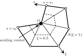
As already mentioned in Section 1, the MK interpolation[24–26] is utilized in this paper to approximate unknown fields in the circumferential direction. The trial functions are independently generated on piecewise smooth edges, which constitute the entire boundary S naturally. It is assumed that a set of scattered nodes si (i = 1,2, …,N) defined by a random function u(s) are distributed on a single edge, where s is the circumferential coordinate. If there are n scattered nodes in the interpolation domain, the function u(s) at point s is approximated in the form


In meshless methods, it is necessary to define the interpolation domain for a point. In this work, the radius of the interpolation domain is calculated as follows:

As shown in Fig.


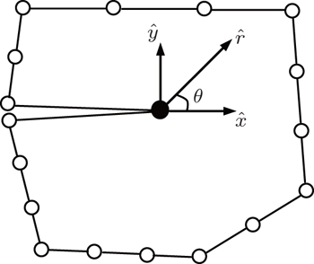
 | Fig. 1. Scaled boundary coordinate system. |
The solution for the extended displacements ū(ξ,s) at any point can be approximated by


By applying the virtual work principle to elastostatics,[28] the scaled boundary meshless equation in extended displacement can be derived as


The homogeneous second-order differential equations in Eq. (


The stiffness matrix


As shown in Eqs. (


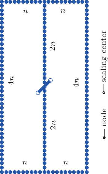
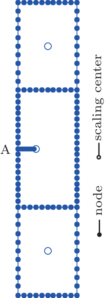
 | Fig. 2. A cracked domain modeled by the scaled boundary node method. |
In order to validate the proposed solution technique, three numerical examples are presented in this section to perform two-dimensional fracture analysis of piezoelectric material. Under the plane strain assumption, the stress and electric displacement intensity factors are computed and compared with other previously reported solutions. In the computation, the piezoelectric materials of PZT-5H and PZT-4 are considered and their elastic, piezoelectric and dielectric constants are given in Table Material constants of piezoelectric materials.
c11
c13
c33
c44
e31
e33
e15
h11
h33
PZT-5H
126
84.1
117
23
−6.5
23.3
17.44
15.03
13.0
PZT-4
139
74.3
115
25.6
−5.2
15.1
12.7
6.45
5.62
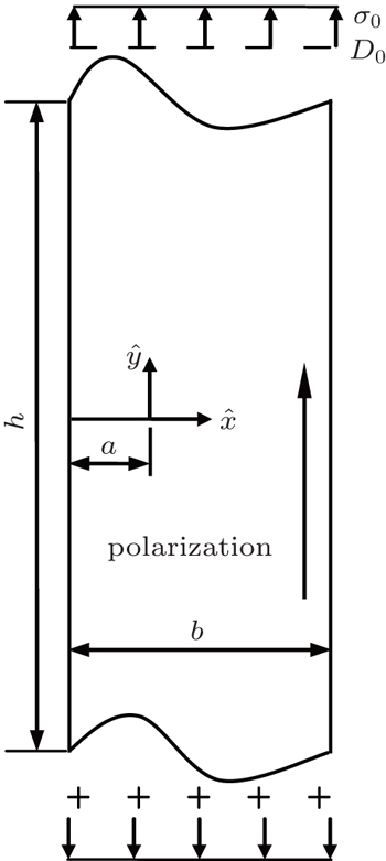
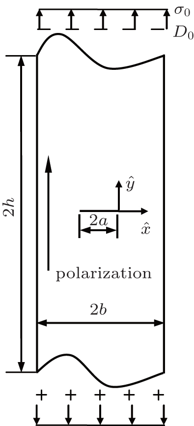
A b × h piezoelectric strip containing an edge crack of length a as shown in Fig.
 | Fig. 3. Piezoelectric strip with an edge crack. |
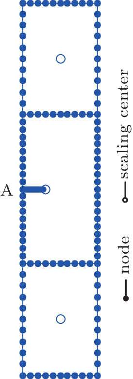
In order to simulate the infinite height, the ratio between the height h and the width b is chosen to be 5, which is relatively large. As shown in Fig.
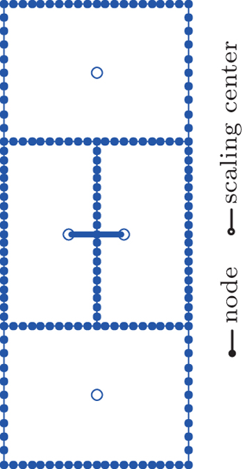
 | Fig. 4. SBNM mesh for the piezoelectric strip with an edge crack. |
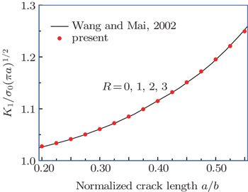
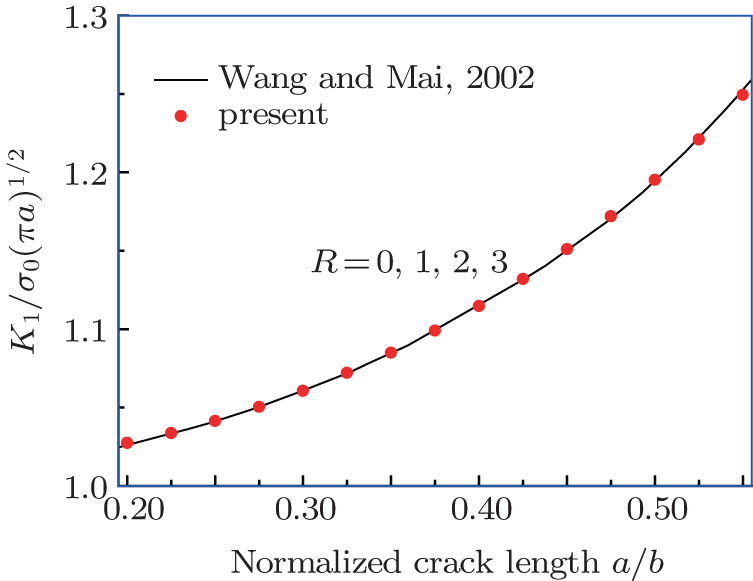
 | Fig. 5. Plots of normalized stress intensity factor KI versus normalized crack length for the piezoelectric strip with an edge crack for different values of R. |
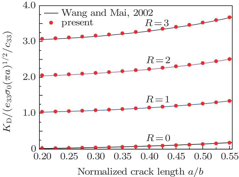
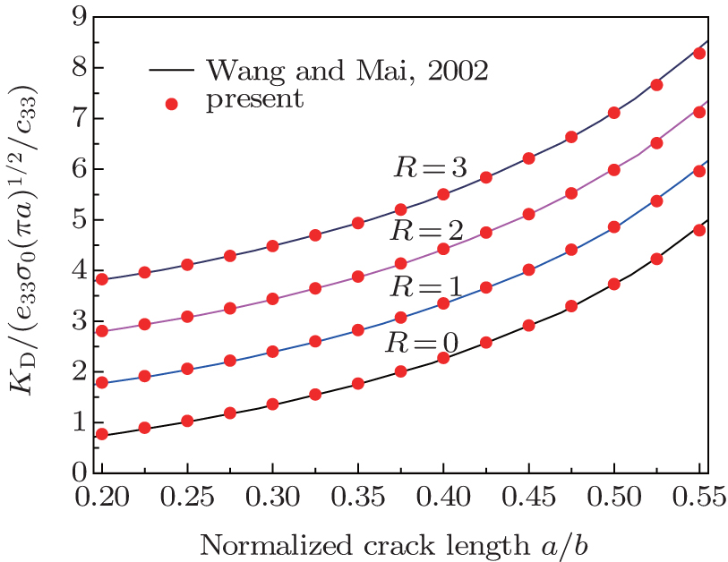 | Fig. 6. Plots of normalized electric displacement intensity factor KD versus normalized crack length for the piezoelectric strip with an edge crack for different values of R. |
The second example deals with a piezoelectric PZT-5H strip of width 2b and height 2h containing a central crack of length 2a. The geometric configuration and the poling direction are shown in Fig.
 | Fig. 7. Piezoelectric strip with a central crack. |
When modeling, this strip is truncated into a finite plate with the height h = 5b. Figure
 | Fig. 8. SBNM mesh for the piezoelectric strip with a central crack. |
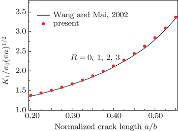
 | Fig. 9. Plot of normalized stress intensity factor KI versus normalized crack length for the piezoelectric strip with a central crack for different values of R. |
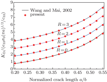
 | Fig. 10. Plots of normalized electric displacement intensity factor KD versus normalized crack length for the piezoelectric strip with a central crack for different values of R. |
A piezoelectric PZT-4 plate of width 2b and height 2h with a θ=45° inclined central crack of length 2a is considered here as depicted in Fig.
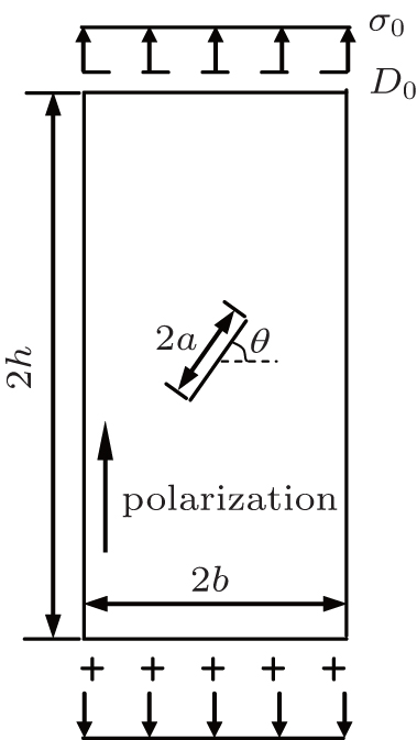 | Fig. 11. An inclined central crack in a rectangular piezoelectric plate. |
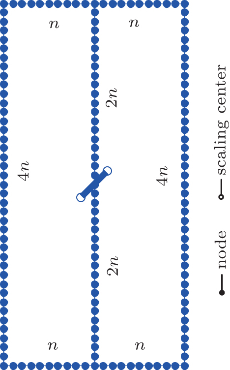 | Fig. 12. SBNM mesh for the piezoelectric plate with an inclined central crack. |
To verify the effectiveness of the present method, the convergence properties are examined by increasing the number of sections in each edge. For different values of n, the normalized intensity factors ahead of the left crack tip are computed under the uniform tension load σ0 and listed in Table
| Table 2. Comparison among normalized intensity factors obtained from different values of n. . |
| Table 3. Comparison among normalized intensity factors for the rectangular plate under σ0. . |
| Table 4. Comparison among normalized intensity factors for the rectangular plate under D0. . |
In this paper, a reliable and efficient solution technique based on the SBNM is extended for fracture analysis in plane piezoelectricity. In the sense of satisfying the equilibrium requirement in the strong form in the radial direction, the SBNM can be viewed as a semi-analytical numerical method. This enables the calculation of the stress and electric displacement intensity factors of piezoelectric materials directly from their definitions without any post-processing. Through the use of the MK interpolation, no mesh generation is necessary and only a nodal data structure on the boundary is required in the SBNM. In comparison with the conventional scaled boundary FEM, the MK interpolation results in superior accuracy, rapid convergence and smooth stress and electric displacement solutions. Besides, it seems that the implementation of the SBNM is convenient because the Kronecker delta property of the MK shape functions can simplify the enforcement of the essential boundary conditions greatly. The results of all the numerical examples demonstrate the effectiveness and robustness of the developed approach to analyzing the two-dimensional fracture problems of piezoelectric materials.