Since an exchange-coupled composite material was proposed by Kneller in 1991,^[1] with a hard phase to provide high coercivity and a soft phase to provide high saturation and remanence, the coercivity, structural, and magnetic properties in permanent magnets have always been an important topic in magnetism.^[2–4] An energy product paradox was proposed in some literatures, which has been intensively studied in both experimental^[5–8] and theoretical^[9–15] works by condensed matter physicists. A lot of works have been devoted to the exploration of the largest energy product experimentally reachable. In 1993, Skomski et al.^[16] proposed that the theoretical energy product (BH)_max of oriented composite magnets could be as large as 120 MG·Oe, which almost doubled that of the best available single-phase permanent magnets.

In order to realize such a giant energy product, many scientists have done a lot of work in the past two decades. A close review shows that the experimental remanence is close to the predicted one, however, the measured coercivity is much smaller.^[17–20] Therefore, such an energy product paradox is intrinsically linked to Brown’s coercivity paradox, i.e., the measured coercivity is much smaller than that predicted by the available theory. Experimentally, huge progresses have been made recently: an energy product (BH)_max of 60 MG·Oe has been obtained in Nd–Fe–B/Fe–Co multilayers by Cui et al.,^[5] while a value of 40 MG·Oe has been reached by Sawatzki et al. in SmCo₅/Fe/SmCo₅.^[21] It is worth noting that at high temperature, the magnetic properties of Nd–Fe–B are inferior to those of Sm–Co due to a lower Curie temperature (about 400 °C against 800 °C), which can occasionally make Sm–Co a better choice compared to Nd–Fe–B.

In the pursuit of the highest energy product reachable, a new structure has been discovered and investigated: the inclusion of an interface layer within bilayers. Choi et al.^[22] found that the maximum energy product of Sm–Co/α-Fe bilayers can be improved by 50% with an intermixed interface layer, and reach a value of 15 MG·Oe. Zhang et al.^[23–25] discovered that by inserting thin non-magnetic spacer layers like Cu in SmCo₅/Fe, increased coercivity and pinning fields can be realized. As a result, (BH)_max jumps from 9 MG·Oe to 32 MG·Oe with a coercivity of 7.24 kOe. The single-phase behavior and the irreversible rotation in the demagnetization process indicates a strong exchange coupling between the Sm(Co, Cu)₅ and Fe layers. Moreover, Liu et al.^[26] discovered that the Fe/Co mixture behavior enhances the interface exchange-coupling and improves the remanence as well as the coercivity of the composite magnet.

In a word, the interface exchange coupling is important in realizing good magnetic properties in Sm–Co/α-Fe layered systems, which, however, have seldom been investigated systematically in theory. In this paper, three-dimensional (3D) micromagnetic simulations and analytical calculations are performed for Sm–Co/α-Fe bilayers, which are then compared to our experimental results. This work focuses on the influence of the exchange coupling and the soft phase thickness on the coercivity and nucleation fields of the system.

Our calculation is based on an exchange-coupled bilayer (see Fig. 1). An o-xyz coordinate system is constructed with the origin located at the center of the interface. The magnetocrystalline axes of both layers and the applied field are assumed to be in the y direction, as shown in Fig. 1.

Fig. 1.

	Figure Option ViewDownloadNew Window
	Fig. 1. Basic scheme of the investigated hard/soft bilayers in the three-dimensional micromagnetic model.

The 3D micromagnetic calculation of the software OOMMF is based on the Landau–Lishitz–Gilbert dynamic equation^[27]

In the 3D simulations, the system is set as a tetragonal box of sizes 300 nm×300 nm×t. The variable t is the thickness of the layers, namely, t = t^h + t^s, as shown in Fig. 1. The subscripts s and h stand for the soft and hard layers, respectively. The thickness of the hard layer t^h is set as 10 nm, while the thickness of the soft layer t^s = 2 nm, 6 nm, and 10 nm. The magnetic structure within these thin layers is discretized into 3 nm × 3 nm × 1 nm cells, which has been optimized to achieve a balance between calculation accuracy and computation time.

In this paper, Sm–Co is chosen as the hard layer, while α-Fe is the soft layer. The material parameters used in the simulation are: M^s = 1.71 × 10³ emu/cc, M^h = 5.5 × 10² emu/cc, K^s = 4.6 × 10⁵ erg/cc, K^h = 5 × 10⁷ erg/cc, A^s = 2.5 × 10⁻⁶ erg/cm, and A^h = 1.2 × 10⁻⁶ erg/cm, which are adopted from Refs. [15], [29], and [30]. Here, A, K, and M denote the exchange energy constant, the anisotropy constant, and the spontaneous magnetization, respectively. Only the exchange interaction between the neighboring region pair is taken into account and the free boundary conditions are chosen. The interface coupling is difficult to describe precisely, as it depends not only on the bulk crystalline structures of the hard and soft layers, but also on the strength of the interface exchange coupling. The exchange energy constant between the soft and hard layers A^hs is set as 1.8 × 10⁻⁶ erg/cm when Sm–Co/α-Fe is in full coupling, while it is taken as 0.9 × 10⁻⁶ erg/cm and 0.45 × 10⁻⁶ erg/cm for low coupling.

The analytical calculation is carried out supposing all layers extending to infinity, which is referred to as the 1D method. The magnetization can be calculated as a function of z, given that the magnetization is uniform within the layer plane (xy plane). The energy density per area in the film plane is^{[15,29,31,32]}

By applying the variational method to the interface exchange coupling energy with suitable boundary conditions, we obtain

In particular, at the nucleation state, the deviation of the magnetization from the applied field direction is small. Thus, the nucleation problem can be solved by an appropriate ansatz or series expansion^[14]

Figure 2(a) shows the calculated hysteresis loops of Sm–Co/α-Fe bilayers for various interface exchange couplings by 3D simulations, where the thicknesses of the hard and soft layers are set as t^h = 10 nm and t^s = 2 nm. It can be seen that the shapes of the hysteresis loops are not sensitive to the exchange coupling between the hard and soft layers, the loops demonstrate a typical exchange-spring magnetic phase for all three values of exchange coupling.^[15,29] As the exchange coupling decreases, the hysteresis loop becomes more slanted, accompanied by a slight decrease of the nucleation field. As A^hs decreases, both pinning and coercive fields increase gradually. On the other hand, the nucleation field decreases, leading to the deterioration of the squareness of the loop. As shown in Fig. 2(a) and summarized in Table 1, the pinning field for A^hs = 4.5 × 10⁻⁷ erg/cm is about 20% larger than that for A^hs = 1.8 × 10⁻⁶ erg/cm. Figure 2(b) shows the calculated hysteresis loops of Sm–Co/α-Fe bilayers for various A^hs based on the 1D calculation, where t^h = 10 nm and t^s = 2 nm. Since for arbitrary applied fields, the angular distribution of θ can be obtained by Eq. (3), and averaging M_scosθ from z = −t^s to t^h, one can obtain the major hysteresis loop for a given hard/soft bilayer. The 1D calculations yield similar loops compared to those obtained by the 3D simulations, justifying our models. As A^hs decreases, both pinning and coercive fields increase gradually whereas the nucleation field decreases, leading to the deterioration of the squareness of the loop. In the meantime, the nucleation field departs from the coercivity and the gap between the two fields enlarges. For all values of A^hs, the pinning field and the coercivity are equal to each other, signifying a coercivity mechanism of pinning.

Fig. 2.

	Figure Option ViewDownloadNew Window
	Fig. 2. Macroscopic hysteresis loops of Sm–Co(10 nm)/α-Fe(2 nm) bilayers obtained by (a) 3D simulations and (b) analytical calculations.

When Sm–Co/α-Fe has an exchange coupling of A^hs = 1.8 × 10⁻⁶ erg/cm, the shape of the hysteresis loop is essentially a rectangle according to the 3D simulations, where the nucleation and pinning fields are close to each other. When A^hs decreases from 1.8 × 10⁻⁶ erg/cm to 4.5 × 10⁻⁷ erg/cm, the gap between nucleation and pinning fields rises from 3.5 kOe to 21 kOe. On the other hand, there is an obvious nucleation point at the applied field of −29.6 kOe for A^hs = 1.8 × 10⁻⁶ erg/cm according to the 1D calculation, which is quite different from the corresponding pinning point at H = −35.8 kOe. This gap between the nucleation and pinning fields rises to 20 kOe as A^hs decreases to 4.5 × 10⁻⁷ erg/cm.

Table 1.

Table 1.

Table 1. Calculated magnetic properties of Sm–Co/α -Fe based on the OOMMF software and 1D calculation, where th = 10 nm. . ts/nm Ahs/10−6erg·cm−1 Method HN/kOe Hc/kOe Hp/kOe Mr/emu·cc−1 2 1.8 1D 30.0 35.8 35.8 743.49 3D 32.69 36.15 36.15 742.46 0.9 1D 27.0 37.2 37.2 743.49 3D 24.49 38.50 38.50 742.46 0.45 1D 22.5 42.5 42.5 743.49 3D 20.01 41.27 41.27 742.46 6 1.8 1D 8.5 15.6 19 985.37 3D 6.65 15.01 15.37 982.99 0.9 1D 7.7 15.4 21.5 985.37 3D 5.75 15.05 21.97 982.99 0.45 1D 6.7 13.95 28.8 985.37 3D 4.91 14.21 27.19 982.99 10 1.8 3D 2.96 8.30 20.51 1043.68 0.9 3D 2.93 6.82 12.60 1043.68

Table 1. Calculated magnetic properties of Sm–Co/α -Fe based on the OOMMF software and 1D calculation, where th = 10 nm. .

As shown in the previous studies,^[13–15,29] the hysteresis loop and the coercivity mechanism are sensitive to the soft layer thickness. Zhao et al. found that as the soft layer thickness increases, the coercivity mechanism changes from nucleation to pinning when the hard layer is large enough. Besides, Asti et al. found that the magnetic phase diagram changes from rigid composite magnet to exchange-spring and finally to decoupled magnet with the increase of the soft layer thickness. Therefore, the hysteresis loops are calculated for various A^hs with t^s = 6 nm, as shown in Fig. 3. Similar to the case with t^s = 2 nm, both pinning and coercive fields go up whereas the nucleation field goes down as A^hs decreases, leading to the deterioration of the squareness of the loop. In contrast with Fig. 2, where the squareness of the loops is quite good, the loops in Fig. 3 demonstrate much worse squareness, in particular for A^hs = 4.5 × 10⁻⁷ erg/cm. Indeed, at this point, the pinning field is about 5.5 times the corresponding nucleation field according to the 3D simulations, demonstrating a typical decoupled magnetic phase.^[15,29] The calculated maximum energy products based on Fig. 3(a) are 38 MG·Oe, 37 MG·Oe, and 35 MG·Oe for A^hs = 1.8 × 10⁻⁶ erg/cm, A^hs = 0.9 × 10⁻⁶ erg/cm, and A^hs = 0.45 × 10⁻⁶ erg/cm, respectively.

Fig. 3.

	Figure Option ViewDownloadNew Window
	Fig. 3. Macroscopic hysteresis loops of Sm–Co(10 nm)/α-Fe(6 nm) bilayers obtained by (a) 3D simulations and (b) analytical calculations.

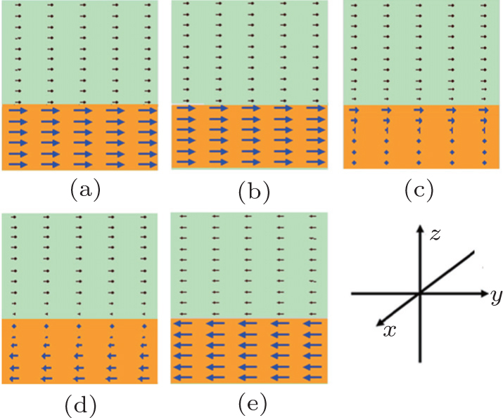
Figure 4 shows the calculated spin configurations in the y–z plane for Sm–Co(10 nm)/α-Fe(6 nm) bilayers with A^hs = 1.8 × 10⁻⁶ erg/cm. The results in Figs. 4(a)–4(e) correspond to the points A–E in the hysteresis loop shown in Fig. 3(a), respectively. The small and large arrows denote the magnetic moments within the Sm–Co and α-Fe layers, respectively, and are proportional to their magnetization. At H = 0 kOe (Fig. 4(a), point A), all the magnetic moments in the system orient parallel to the y axis. At H = −7.0 kOe (Fig. 4(b), point B), the magnetization begins to deviate from the previous saturation state incoherently. At H = −12.0 kOe (Fig. 4(c), point C), one can find that the magnetic moments in the α-Fe layer far away from the interface have rotated 90°, while those near the interface are pinned by the exchange coupling with the Sm–Co layer. When the applied field decreases to −15.0 kOe (Fig. 4(d), point D), most magnetic moments in the α-Fe layer have reversed, while the magnetic moments in the Sm–Co layer far away from the interface have hardly rotated due to the large crystalline anisotropy, forming a 180° domain wall at the interface. At H = −16 kOe (Fig. 4(e), point E), the magnetic moments in both hard and soft phases have reversed completely.

Fig. 4.

	Figure Option ViewDownloadNew Window
	Fig. 4. 2D evolution of the magnetization calculated by OOMMF for Sm–Co(10 nm)/α-Fe(6 nm) with exchange coupling Ahs = 1.8 × 10−6 erg/cm: (a) H = 0 kOe, magnetization saturation, (b) H = −7.0 kOe, near nucleation field, (c) H = −12.0 kOe, between the nucleation and coercive fields, (d) H = −15.0 kOe, the coercive field, (e) H = −16.0 kOe, the pinning point.

Experimentally, the interface of the hard/soft layers has been intensively modified to obtain the best performance for the exchange spring film. A spacing layer Ta was inserted between Nd₂Fe₁₄B and FeCo layers to adjust the exchange coupling and magnetostatic interaction to obtain the largest (BH)_max in NdFeB-based nanocompiste films.^[5] For the SmCo/Fe system, a diffusion layer was reported to be effective for getting a larger nucleation field and hence (BH)_max.^[6] A Cu layer was used in multilayer films Cr(50 nm)/[SmCo₆(9 nm)/Cu(x nm)/Fe(5 nm)/Cu(x nm)]₆/Cr(100 nm)/SiO₂ (x = 0–0.75) and a high (BH)_max of 32 MG·Oe was obtained by some of us.^[23–25] Although the Cu layer promotes the crystallization of the SmCo phase to form a uniform multilayer, the Cu layer with different thickness is considered to adjust the exchange coupling as well. In the case of the SmCo layer directly contacting the Fe layer, the exchange coupling is strong. With the Cu thickness increased, the soft and hard phases are separated by the Cu layer, which results in a decrease of the exchange coupling. Figure 5 demonstrates the measured hysteresis loops of two SmCo/Cu/Fe multilayers at 10 K and the calculated loops based on OOMMF. It can be observed that the trend of the experimental loops (with the Cu layer thickness increasing from 0 to 0.75 nm) is consistent with that of the calculated loops (with A^hs decreasing from 1.8 × 10⁻⁶ erg/cm to 0.9 × 10⁻⁶ erg/cm). The smoothness and two-stage feature in the calculated loops are due to the ideal material parameters adopted in the calculation, while in experiment, the more complicated polycrystalline structure, dispersion in the composition, and defects exist, therefore the intrinsic property of the material is affected. Nevertheless, our calculation data show qualitative agreement with the experiment one.

Fig. 5.

Figure Option ViewDownloadNew Window

Fig. 5. Comparison of calculated hysteresis loops with experimental loops for Cr(50 nm)/[SmCo6(9 nm)/Cu(x nm)/Fe(5 nm)/Cu(x nm)]6/Cr(100 nm)/a-SiO2 (x = 0–0.75). (a) The black squares are for the sample with x = 0 annealed at 500 °C measured at 10 K while the red circles are for the sample with x = 0.75 annealed at 500 °C measured at 10 K. (b) The black lines are for th = 9 nm, ts = 5 nm, and Ahs = 1.8 × 10−6 erg/cm; while the red lines are for th = 9 nm, ts = 5 nm, and Ahs = 0.9 × 10−6 erg/cm using OOMMF.

Figure 6 demonstrates the angular distributions of magnetization in the +z direction for Sm–Co (10 nm)/α-Fe (2 nm) bilayers with identical exchange coupling A^hs = 0.45 × 10⁻⁶ erg/cm based on 1D and 3D models. In the analytical model, the angular distributions of magnetization in the z direction can be obtained by minimizing the energy density expressed in Eq. (3), which is coherent in the x–y plane. With the 3D calculation, the angular distributions are obtained by averaging the component of all the magnetic moments in the applied field direction with a certain z.

Fig. 6.

	Figure Option ViewDownloadNew Window
	Fig. 6. Calculated spatial distributions of magnetization direction for Sm–Co(10 nm)/Fe(2 nm) bilayers based on (a) analytical calculations and (b) 3D simulations with exchange coupling Ahs = 0.45 × 10−6 erg/cm.

As shown in Fig. 6(a), a small deviation of the magnetization from the previous saturation state occurs at H = −22.6 kOe, which is called nucleation according to Brown. Under this field, a 7.11° infant domain wall has been formed with θ^h = 0°, θ⁰⁺ = 2.98°, θ⁰⁻ = 6.26°, and θ^s = 7.11°. The domain wall grows fast as the applied field reduces. When the applied field reaches H = −35.2 kOe, a 110° domain wall forms. Further decrease of the applied field leads to a faster growth of the domain wall. At the coercive point, it reaches its maximum with a value of 136° when the applied field drops to −42.5 kOe. Additional decrease of the applied field will result in the magnetic reversal of the whole bilayer system. In Fig. 6, the 3D simulation and the 1D calculation show the same results.

From the above discussion, one can find that a large nucleation field is essential to keep the squareness of the corresponding hysteresis loop. In this section, the dependence of this critical field on the exchange interaction and the soft layer thickness is discussed. In nanocomposite films, the hard phase offers a high anisotropy to produce the high coercivity, but this effect strongly depends on its thickness. If t^h is smaller than the corresponding Bloch wall width,^[14,30] which is about 4.9 nm for Sm–Co, its magnetization will be easily reversed by the soft phase through the exchange interaction. While if t^h is large enough, the magnetic properties will not depend on it.^[33] Therefore, in the calculation below, the thickness of the hard phase is set to 10 nm, which is larger than the Bloch wall width.

Figure 7 and Table 1 demonstrate the calculated nucleation fields for various exchange interactions and soft film thicknesses based on Eq. (6). For comparison, the hysteresis loops in the case of t^s = 2 nm are calculated using 3D OOMMF and the 1D method, and the nucleation fields are obtained from the loops. One can find that the three methods yield roughly the same nucleation fields. When A^hs approaches 0, H_N comes close to 0.53 kOe, i.e., the nucleation field of the single α-Fe phase, and at this point, the system degenerates into a typical decoupled magnetic system. With increased exchange interactions, H_N increases and approaches some constant value for large A^hs, which refers to the case of an infinite exchange coupling A^hs = ∞. In the case of a constant exchange interaction, H_N increases when the soft layer thickness decreases.

Fig. 7.

	Figure Option ViewDownloadNew Window
	Fig. 7. Calculated nucleation field as a function of the exchange coupling Ahs. The solid lines are obtained with Eq. (6). The dashes are calculated with 1D and 3D models.

The nucleation field as a function of the thickness of the α-Fe layer under various exchange interactions A^hs is shown in Fig. 8. The value of 180 kOe is found when d_Fe = 0, which is close to the anisotropy field of Sm–Co (181.8 kOe). The nucleation field decreases when d_Fe increases, the strong decline in the region from d_Fe = 0 nm to ∼4 nm is in accordance with the theoretical predictions of Leineweber,^[32] Zhao,^[34,35] and other numerical simulations.^[29,36] From d_Fe = 0 nm to 10 nm, the nucleation fields with a strong exchange coupling are always larger than those with a weak coupling. A large gap exists between d_Fe ≈ 0.5 nm and d_Fe ≈ 5.0 nm. In the case of A^hs = 1.8 × 10⁻⁶ erg/cm, the nucleation fields and coercivities obtained by the 1D method and 3D OOMMF are shown in Fig. 8 as well. When t^s is smaller than 1.0 nm, the loops are rectangular and the nucleation fields are equal to the coercivities or pinning fields; this thickness is denoted as the first critical thickness,^[34] which can be estimated by t_crit1 = π (A^s/2K^h)^1/2.^[1] Using analytical micromagnetics, Zhao et al. found that the first critical thickness is inversely proportional to the square root of the magnetocrystalline anisotropy constant of the hard phase, which is consistent with the above formula. With d_Fe larger than 1.0 nm, the nucleation and coercive fields deviate and the hysteresis loop gradually loses its squareness.^[34,35]

Fig. 8.

	Figure Option ViewDownloadNew Window
	Fig. 8. Calculated nucleation and coercive fields as a function of the soft layer thickness ts. The solid lines are obtained with Eq. (6). The dashes are calculated with 1D and 3D models.

The effects of the exchange coupling on magnetic properties were investigated for Sm–Co/α-Fe bilayers using a 3D micromagnetic software OOMMF and a 1D analytical model. A reduced exchange coupling results in lower nucleation fields and higher coercivities. Both methods show agreeable results with the experimental multilayer data. On the other hand, when the soft layer thickness increases, both pinning field and remanence increase whereas the nucleation and coercive fields decrease, leading to the deterioration of the squareness of the loops. The calculated results can partially explain Brown’s coercivity paradox in hard/soft composite materials. A strong exchange coupling is essential to keep the squareness, therefore a large energy product.