The excitation process has been studied since the foundation of quantum mechanics, and perturbation theory and numerical solution of Schrödinger equation are the two main theoretical methods to study the resonant excitation process.^[1–3] The two methods are both based on the quantum theory of the Copenhagen School which describes electronic state via the concept of probability.^[4–6] Copenhagen school abandons the concept of trajectory, and as a result, the excitation process of electrons from the ground state to the first excited one can only be described through the concept of probability rather than that of trajectory.

Recently, Bohmian mechanics method has attracted increasing attention,^[7–10] for this method has obvious advantages in describing the interaction between the intense laser pulses and atoms as well as molecules,^[11–19] through which a more intuitive understanding of the strong field physics can be obtained via the detailed analysis of the “classical” mechanical quantities, including trajectory, force, and energy.^[20–31] An excited state is a quantum state whose energy is higher than the ground state of atom and molecule or cluster. Irradiated by the laser pulse resonant with the ground and first excited states of the atom, the electron in the ground state can be excited to the first excited state thoroughly as the pulse area is appropriate.^[32–34] When the electron is subject to a laser pulse with long period and low intensity, and its frequency is the resonance frequency between the ground state and first excited state, electron can be excited to first excited state completely. The traditional quantum mechanics can only present the temporal evolution of the probability of each state of electron. In our work, utilizing the Bohmian mechanics method, we can describe the electronic excitation process from the ground state to the first excited one starting from the particulate nature of electron.

To study excitation process simply, we select one-dimensional model of single electron. Under the dipole approximation in the length gauge, the time-dependent Schrödinger equation (TDSE) that describes the interaction between strong laser pulse and atom is given by (atomic units are used throughout, unless otherwise stated)

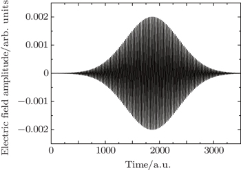
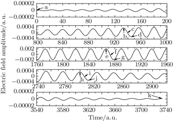
We choose a laser field whose peak amplitude, central frequency, and duration are 0.002 a.u., 0.2693 a.u., and 160 optical cycles, and this laser field can fully stimulate the excitation of electron from ground state to first excited state, as shown in Fig. 2. Here, 0.2693 a.u. is the energy difference between the ground state and the first excited state. We can see from Fig. 2 that under the irradiation of this laser filed, the electrons can be excited from the ground state to the first excited state completely. In the following part, we will study the physical model by the Bohmian mechanics method.

Fig. 1.

	Figure Option ViewDownloadNew Window
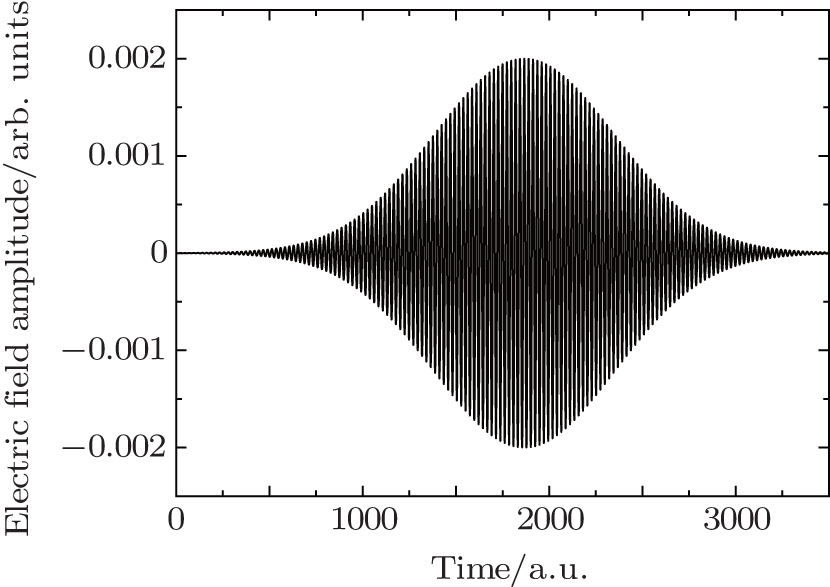
	Fig. 1. Time evolution of laser field whose peak amplitude, central frequency, and duration are 0.002 a.u., 0.2693 a.u., and 160 optical cycles, respectively.

Fig. 2.

	Figure Option ViewDownloadNew Window
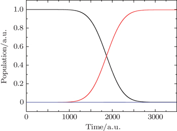
	Fig. 2. Time evolution of the population of ground state (black curve), first excited state (red curve), and other excited states (blue curve) under the action of the laser field shown in Fig. 1.

To illustrate that the energy calculated by the Bohmian mechanics method is still consistent with that obtained by numerically solving the TDSE, we present in Fig. 3 the average energy of 2000 Bohmian particles (red curve) and the average energy of the TDSE calculation (black curve) and make a comparison between them. In this model, the energy of the ground state is −0.503 a.u., and that of the first excited state is −0.2693 a.u. From Fig. 3, it can be seen that in the excitation process, the average energy of 2000 Bohmian particles and that obtained by numerically solving the TDSE are in good agreement with each other, indicating that we can utilize the energy of Bohmian particles to analyze the excitation process.

Fig. 3.

	Figure Option ViewDownloadNew Window
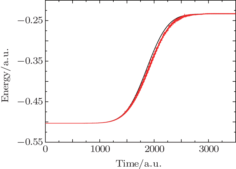
	Fig. 3. Temporal evolution of the statistical average of the total energy of 2000 Bohmian particles (red curve) and that of average energy of electron calculated from the TDSE (black curve).

In order to better study the excitation process, we also present the evolution of the electronic wave-packet dynamics, and the corresponding Bohmian trajectories, as shown in Fig. 4. It can be seen from the figure that the calculated Bohmian trajectories (see Fig. 4(b)) is consistent with the evolution of electronic wave-packet calculated from the TDSE (see Fig. 4(a)).

Fig. 4.

	Figure Option ViewDownloadNew Window
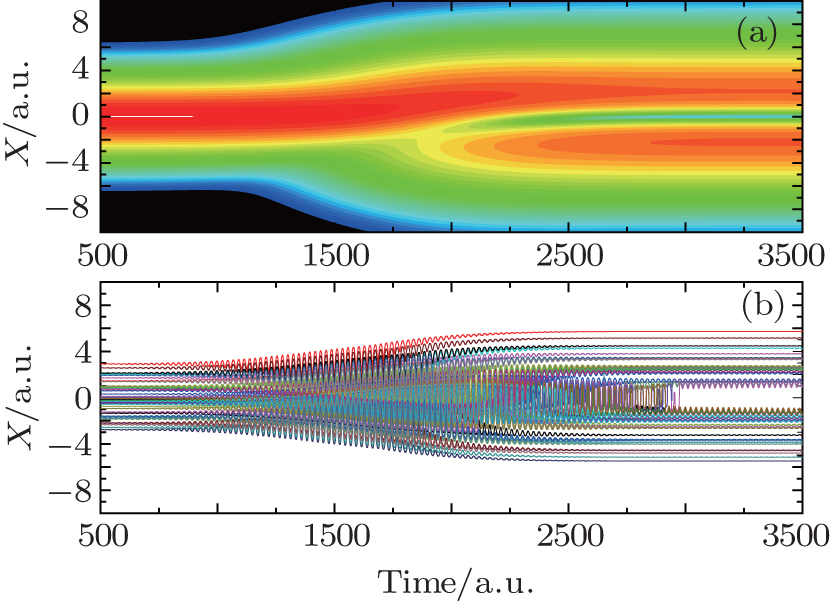
	Fig. 4. Excitation process of electrons in the laser pulse whose duration is 160 optical cycles. (a) Probability density of the electron obtained by numerically solving the TDSE; (b) Bohmian trajectories calculated by the Bohmian mechanics.

Fig. 5.

	Figure Option ViewDownloadNew Window
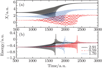
	Fig. 5. Time evolution of (a) trajectory, (b) energy of three typical bohemian particles whose initial positions are 2.91 (solid black curve), 1.70 (dotted blue curve), 0.59 (dashed red curve), respectively.

We choose three typical Bohmian particles whose initial positions are 2.91, 1.70, and 0.59, respectively. It is obvious that the Bohmian particle far away from the nucleus (solid black curve) is easier to be excited, and its excitation time is around 1688.93; in contrast, the Bohmian particle near the nucleus is excited after a moment (dashed red curve), and its excitation time is around 2363.23. Therefore, we can say that the Bohmian particles far away from the nucleus are easier to be excited, and are excited firstly.

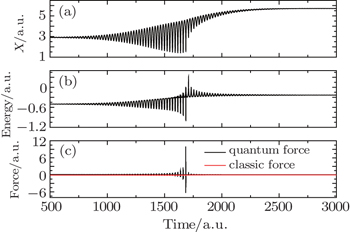
We choose one of the Bohmian particles to analyze its excitation process, as shown in Fig. 6. It can be seen from Fig. 6(a) that the oscillation amplitude of the trajectory increases (decreases) with the increase of time gradually before (after) t = 1685. We see from Fig. 6(c) that the particle is free from the classical force and only feels the quantum force. It can be seen from Figs. 6(b) and 6(c) that under the action of quantum force, the energy of Bohmian particle fluctuates around the value of the ground state’s energy before t = 1685, rises abruptly due to the strong quantum force at t = 1685, and fluctuates around the value of the first excited state’s energy after t = 1685, getting close to the energy of first excited state gradually. From the perspective of trajectory, energy, and force, the moment shows obvious characteristic of abrupt change, which can be taken as the criterion of excitation. Therefore, we can say that the excitation is not a slowly changing process but an abruptly changing one, and the main factor leading to excitation is the quantum force rather than the classical force.

Fig. 6.

	Figure Option ViewDownloadNew Window
	Fig. 6. Excitation process of one Bohmian particle whose initial position is 2.9. (a) Trajectory, (b) energy, and (c) force.

We select 11 typical instants from Fig. 1, as shown in Fig. 7, where a and k are the starting point and ending point of the electric field; b, e, and h correspond to the peak of electric field; c, f, and i are the instants when the amplitude of the electric field is zero; and d, g, and j correspond to the peak amplitude when the direction of the electric field is reverse. b, c, and d are around T/4, e, f, and g are around T/2, and h, I, and j are around 3T/4. In the following part, we will take a look at the distribution of these Bohmian particles at those typical instants.

Fig. 7.

	Figure Option ViewDownloadNew Window
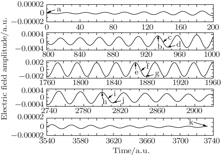
	Fig. 7. Amplified electric field shown in Fig. 1. Eleven typical instants are selected, i.e., a, b, c, d, e, f, g, h, i, j, and k.

From Fig. 8, we find that when the electric field strength is 0, the Bohmian particles in the ground state do not move (see Fig. 8(a)). As the time evolves to the vicinity of 1/4T, the electric field strength increases to the value shown by instant b, and the energy of Bohmian particle changes tinily, as shown in Fig. 8(b). When the electric field strength is 0, the corresponding energy range of Bohmian particles is widened (see Fig. 8(c)). In addition, the energy of Bohmian particles on the negative half axis is higher and that on the positive one is lower. When the strength of the laser field is maximum in the reverse direction, i.e., at instant d, the Bohmian particles return to the state at instant b.

Fig. 8.

	Figure Option ViewDownloadNew Window
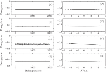
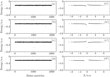
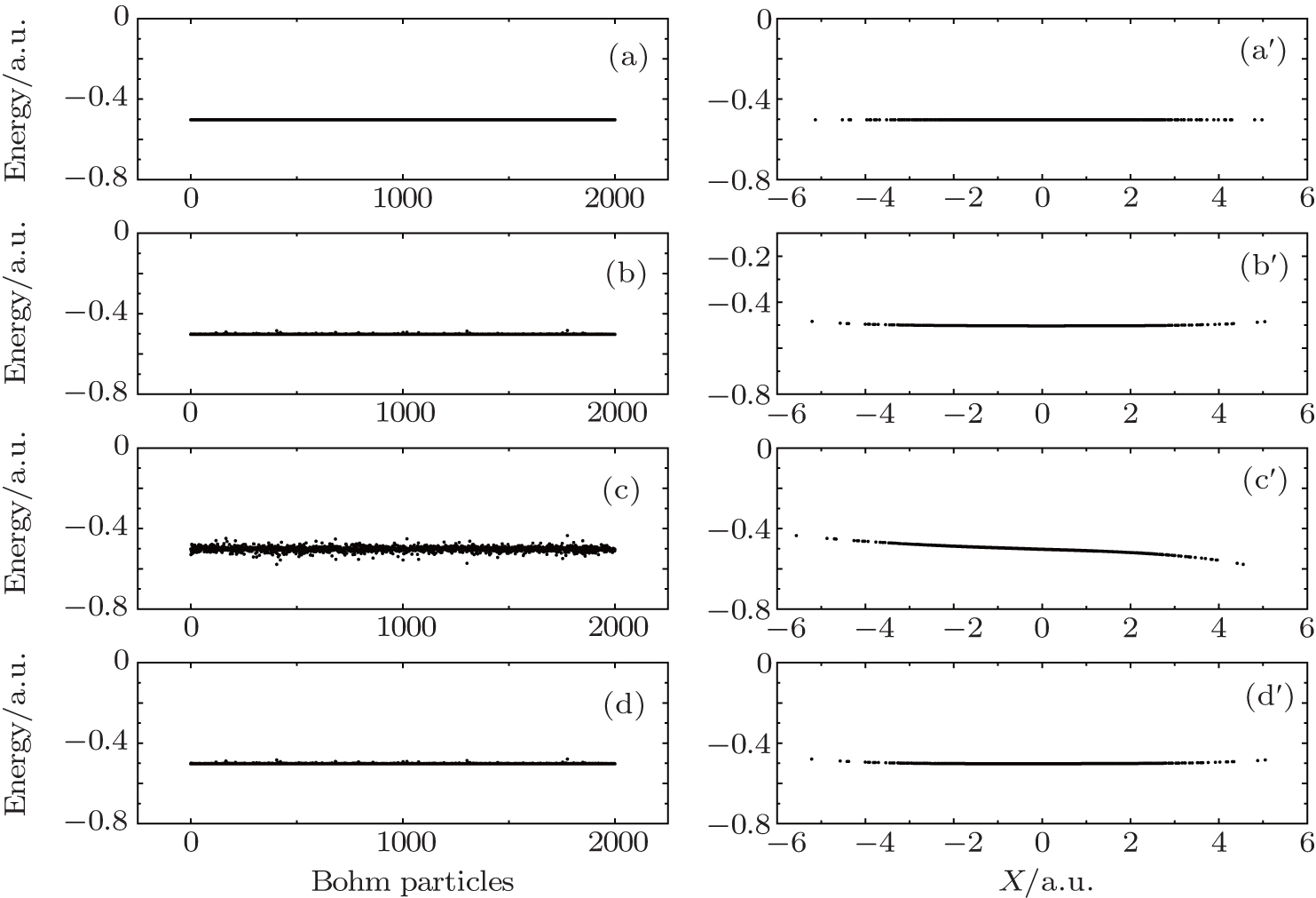
	Fig. 8. Relationship between energies and spatial positions of 2000 Bohmian particles. Panels (a), (b), (c), (d) and (a′), (b′), (c′), (d′) correspond to the four instants a, b, c, d shown in Fig. 7.

Here, we select two typical particles to explain the above phenomena: one is from the center of nuclear region, and the other one is from the edge of nuclear region whose initial positions are 2.91 and 0.01, respectively. In Fig. 9, we present the excitation process of the two Bohmian particles during the period b–d. It can be seen from Fig. 9(a) that during this period, the trajectory of the Bohmian particle in the nuclear region has hardly any change (solid red curve); whereas the trajectory of the Bohmian particle far away from the nuclear region deviates slightly at instant c and return to the initial position at instant d (solid black curve). From Fig. 9(c), we can see that during the period b–d, the force that the Bohmian particle in the nuclear region feels is close to zero, while the Bohmian particle far away from the nuclear region is subject to a tiny total force, resulting in the slight deviation of its trajectory. Consequently, the phenomena shown in Fig. 9(a) can be well understood, and it is the slight deviation of Bohmian particle’s trajectory that leads to the spatial asymmetry phenomenon shown in Fig. 8(c′). Next, we will analyze the mechanism underlying the broadening of the energy band. It can be seen from Fig. 9(b) that the energy of the Bohmian particle in the nuclear region undergoes hardly any change (solid red curve); while the energy of the Bohmian particle far away from the nuclear region changes largely (solid black curve). This effect can be attributed to the fact that the Bohmian particle far away from the nuclear region is subject to a tiny total force, and thus its position deviates, leading to the variation of its total energy. That is to say, both the broadening of energy band and the asymmetry of Bohmian particles’ spatial positions result from the fact that the quantum force of the Bohmian particle far away from the nucleus feels is a little larger than the classical force.

Fig. 9.

	Figure Option ViewDownloadNew Window
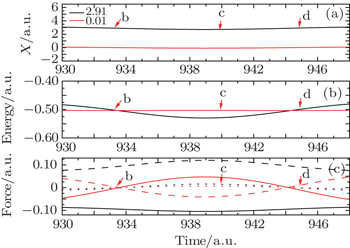
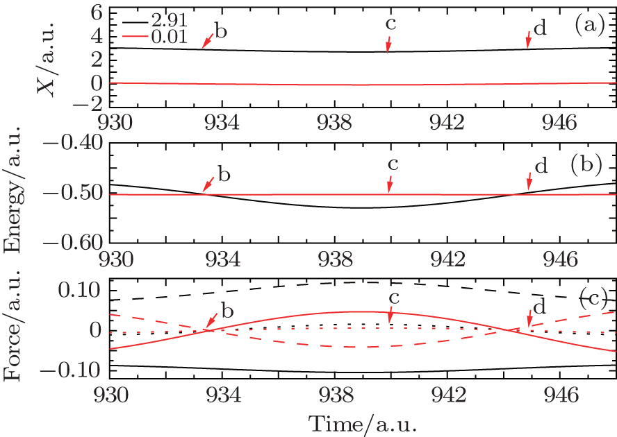
	Fig. 9. (a) Trajectories, (b) energies, and (c) forces of the two Bohmian particles whose initial positions are 2.91 (solid black curves) and 0.01 (solid red curves) during the period b–d shown in Fig. 7. The solid, dashed, and dotted curves in panel (c) denote the classical, quantum, and total forces.

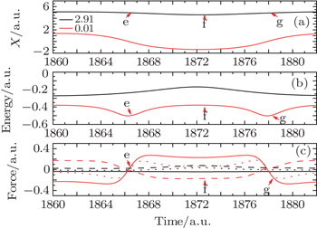
As the amplitude of the electric field reaches the peak value 0.002 a.u., i.e., around the moment 1/2T, three typical instants, i.e., e, f, and g are chosen. These three instants correspond to three different electric field strengths, as shown in Fig. 7. When the amplitude of electric field is 0.002 a.u., we find that a uniform energy band is formed by 2000 Bohmian particles (see Fig. 10(a)), and its spatial distribution is symmetric, as shown by Fig. 10(a′). All the Bohmian particles are centered on the nucleus, the farther away from the nucleus, the higher the energies of Bohmian particles are, and vice versa; when the amplitude of the electric field becomes 0 (instant f), the energy band is no longer uniform (see Fig. 10(b)) and the spatial distribution of particles is asymmetric (see Fig. 10(b′)); when the amplitude of the electric field reaches its maximum value in the reverse direction, the energy band becomes uniform (see Fig. 10(c)), and the spatial distribution of particles become symmetric again (see Fig. 10(c′)).

Fig. 10.

	Figure Option ViewDownloadNew Window
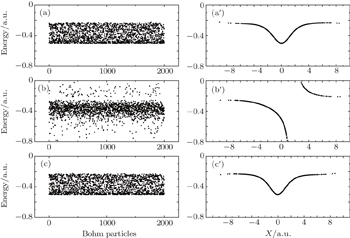
	Fig. 10. (a), (b), (c) and (a′), (b′), (c′) correspond to the three instants e, f, g shown in Fig. 7. They show the relationship between the energies and spatial positions of 2000 Bohmian particles.

We still utilize the two Bohminan particles to analyze the phenomena shown in Fig. 10, and present in Fig. 11 their excitation process during the period e–g. It can be seen from Fig. 11(a) that during this period, the trajectory of the Bohmian particle far away from the nuclear region does not change much (solid black curve), while that of the Bohmian particle in the nuclear region changes greatly (solid red curve), which can be attributed to the fact that the total force that the Bohmian particle far away from the nuclear region feels is relatively tiny (solid black curve in Fig. 11(c)), while the total force that the Bohmian particle in the nuclear region feels (mainly comes from the larger Coulomb force) is relatively large, as shown in Fig. 11(c). The drastic change of the spatial positions of particles results in the drastic change of their Bohmian energies (see Fig. 11(b)), thereby generating the relatively broad energy band, as shown in Figs. 10(e)–10(g). It is the fact that the Coulomb force of the Bohmian particle in the nuclear region feels is larger than the quantum force that leads to the generation of such structure.

Fig. 11.

	Figure Option ViewDownloadNew Window
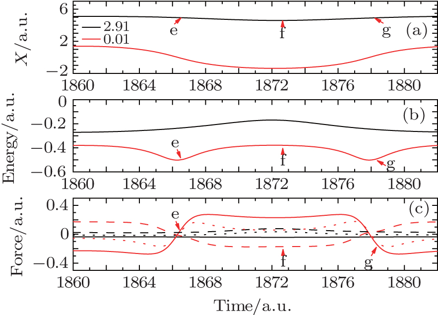
	Fig. 11. (a) Trajectories, (b) energies, and (c) forces of the two Bohmian particles whose initial positions are 2.91 (solid black curves) and 0.01 (solid red curves) during the period e–g shown in Fig. 7. The solid, dashed, and dotted curves in panel (c) denote the classical, quantum, and total forces.

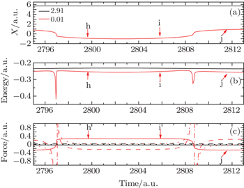
Around the moment 3/4T, we select three typical instants, i.e., h, i, and j, as shown in Fig. 7. In practice, undergone the process shown in Fig. 10, the Bohmian particles have already completed the excitation process basically, for these particles are generally in first excited state and there is a gap in the vicinity of the nuclear region. By comparing the results at instant h (see Figs. 12(a) and 12(a′)) and i (Figs. 12(b) and 12(b′)), we find that as the amplitude of the electric field evolves to zero, the energy and the spatial position of Bohmian particles change little, and the only difference is that the gap formed by Bohmian particles near the nuclear region becomes a little larger at instant i. When the direction of electric field is reverse (e.g., at instant j), only the position of Bohmian particle near the nuclear region changes, and the energy and the position of Bohmian particle that on both sides of the nuclear region are basically stable, as shown in Figs. 12(c) and 12(c′). Finally, at the end of the electric field, i.e., at instant k, the energy of all Bohmian particles is basically stable, indicating that the electronic excitation process has been completed, as shown in Figs. 12(d) and 12(d′).

Fig. 12.

	Figure Option ViewDownloadNew Window
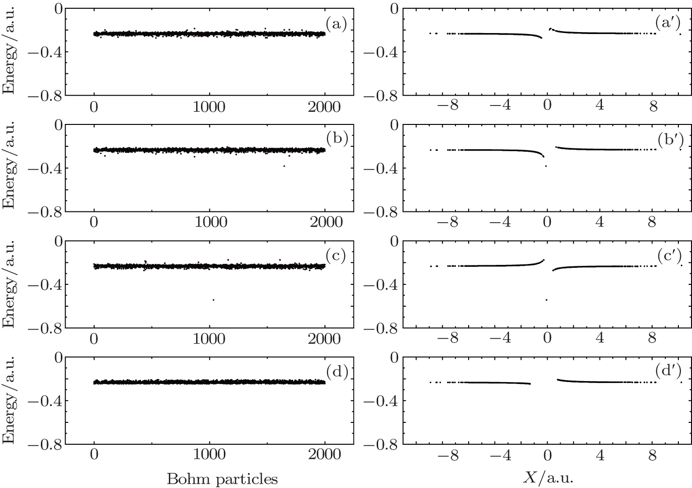
	Fig. 12. (a), (b), (c), (d) and (a′), (b′), (c′), (d′) correspond to the four instants h, i, j, k shown in Fig. 7. They show the relationship between the energies and spatial positions of 2000 Bohmian trajectories.

Figure 13 shows the excitation process of the two typical Bohmian particles during the period h–j. We can see from Fig. 13(a) that the trajectory of the Bohmian particle far away from the nuclear region has hardly any change (see the solid black curve), and its energy is stable (solid black curve in Fig. 13(b)), which can be attributed to the fact that the total force acting on it is zero; in contrast, for the Bohmian particle in the nuclear region, its trajectory changes periodically, and although its energy changes abruptly as several instants, it remains stable at other times, as shown in Fig. 13(b). It can be seen from Fig. 11(c) that around the instants 2797 and 2809, the Bohmian particle feels a large quantum force, and it is this quantum force that leads to the abrupt change of its trajectory. As a result, during the period h–j, along with the change of the direction of the laser field, the spatial position of the Bohmian particle in the nuclear region changes.

Fig. 13.

	Figure Option ViewDownloadNew Window
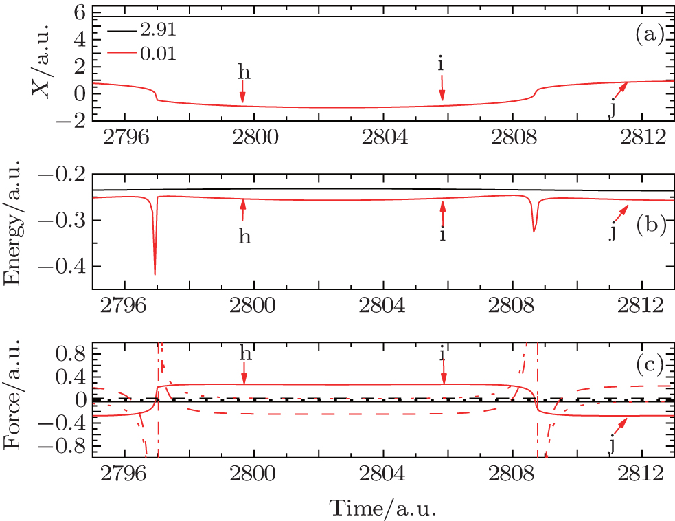
	Fig. 13. (a) Trajectories, (b) energies, and (c) forces of the two Bohmian particles whose initial positions are 2.91 (solid black curves) and 0.01 (solid red curves) during the period h–j shown in Fig. 7. The solid, dashed, and dotted curves in panel (c) denote the classical, quantum, and total forces.

In this paper, we utilize the Bohmian mechanics method to describe the electronic excitation process from the angle of the trajectory. It is found that the excitation process is not a slowly changing process, but an abruptly changing one, which can be attributed to the fact that the Bohmian particle is subject to a strong quantum force at several specific moments. We also give the energy and position of Bohmian particles at several typical instants and make a detailed analysis for the dynamical process so as to make it intuitive to understand the excitation process.