


Hysteresis-induced bifurcation and chaos in a magneto-rheological suspension system under external excitation
[Zhang Hailong1, 2, Wang Enrong2, Min Fuhong2, Zhang Ning1, †,  ]
]
]
|
|


† Corresponding author. E-mail:
Projects supported by the National Natural Science Foundation of China (Grant Nos. 51475246, 51277098, and 51075215), the Research Innovation Program for College Graduates of Jiangsu Province China (Grant No. KYLX15 0725), and the Natural Science Foundation of Jiangsu Province of China (Grant No. BK20131402).
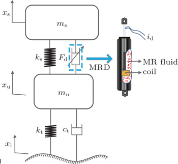
The magneto-rheological damper (MRD) is a promising device used in vehicle semi-active suspension systems, for its continuous adjustable damping output. However, the innate nonlinear hysteresis characteristic of MRD may cause the nonlinear behaviors. In this work, a two-degree-of-freedom (2-DOF) MR suspension system was established first, by employing the modified Bouc–Wen force–velocity (F–v) hysteretic model. The nonlinear dynamic response of the system was investigated under the external excitation of single-frequency harmonic and bandwidth-limited stochastic road surface. The largest Lyapunov exponent (LLE) was used to detect the chaotic area of the frequency and amplitude of harmonic excitation, and the bifurcation diagrams, time histories, phase portraits, and power spectrum density (PSD) diagrams were used to reveal the dynamic evolution process in detail. Moreover, the LLE and Kolmogorov entropy (K entropy) were used to identify whether the system response was random or chaotic under stochastic road surface. The results demonstrated that the complex dynamical behaviors occur under different external excitation conditions. The oscillating mechanism of alternating periodic oscillations, quasi-periodic oscillations, and chaotic oscillations was observed in detail. The chaotic regions revealed that chaotic motions may appear in conditions of mid-low frequency and large amplitude, as well as small amplitude and all frequency. The obtained parameter regions where the chaotic motions may appear are useful for design of structural parameters of the vibration isolation, and the optimization of control strategy for MR suspension system.
Magneto-rheological fluids (MRFs) are known as smart materials, whose yield stress and viscosity can reversely change when subjected to or removed from a magnetic field.[1–4] The MR damper (MRD) utilizing MRF has highly controllable yield stress, which allows the MRD for the adaption to a wide range of shock loads and vibrations. Moreover, MRD possesses the characteristics of low power consumption and fast response, because the controllable output damping force can be easily achieved by adjusting the DC drive current. Therefore, MRDs have been widely used in the semi-active structural control applications.[5–8] However, like most of the advanced devices adopting smart materials (such as ionic polymer metal composites, piezoelectrics, and shape memory alloys), MRDs also exhibit hysteresis nonlinear properties. The multi-valued and non-smooth hysteresis will bring up many complex dynamical behaviors, such as bifurcation and chaos.[9,10] Walter[11] investigated the responses and codimension-one bifurcations in masing-type and Bouc–Wen hysteretic oscillators, and found a rich class of solutions and bifurcations mostly unexpected for the hysteretic loop. Lamarque[12] investigated the dynamics of energy harvesting systems with hysteresis and nonlinearity, where the hysteresis bifurcations were explained. Nicola[13] carried out the study on a short steel wire rope which exhibited the hysteresis, and found that the Neimark–Sacker bifurcations cause the loss of stability of the periodic response.
In engineering application, most effort was made on the semi-active control of MRDs, and the 2 degree of freedom (2-DOF) MR suspension system is a pervasive solution for the control strategy design. In Ref. [5], the skyhook semi-active controller, which was derived from the 2-DOF MR suspension model, was employed on a seat suspension for a helicopter crew seat. In Refs. [6] and [7], the 2-DOF MR suspension system was employed on the vehicle semi-active suspension system, to simultaneously satisfy the performance requirements of ride comfort and handling stability. However, there are few studies on the nonlinear dynamic behaviors caused by hysteresis, especially little on the 2-DOF MR suspension system. Raghavendra[14] examined the chaotic motion in a vehicle suspension system with hysteretic nonlinearity when excited by a road profile, thus establishing the limiting conditions of the MR suspension system. Luo et al.[15] modeled the 1-DOF semi-active MR suspension system through a piecewise-linear model. The mapping technique was employed to predict the periodic motions and bifurcation, and the periodic and stable motions were carried out. Krzysztof[16] proposed the nonlinear MR damping force by a hyperbolic tangential function, thereby building the MR damped Duffing system. Regions of stable or unstable solutions have been determined by a continuation method. Yan[17] investigated the effect of nonlinear damping suspension on the nonperiodic motions of a flexible rotor in journal bearings, and found more complicated nonlinear damping effects than those in the Duffing oscillators. Litak[18] investigated the chaotic motion in a hysteresis nonlinear vehicle suspension system, which was subjected to multi-frequency excitation, and found the critical amplitude of the road surface when the system vibrates chaotically. Nevertheless, the Bouc–Wen phenomenon model is a recognized model to describe MRDs, which accurately represents the inherent hysteresis nonlinear properties, compared with both a piecewise-linear model and the hyperbolic tangential model.[19] Though the Bouc–Wen model is widely used in practical application, the nonlinear dynamic analysis of MR suspension based on it is still rare. In addition, stability analysis under a random road spectrum is more practical and applicable, but it was ignored in the previous studies.
Due to the complex and nonlinear hysteretic characteristics of MRDs, intensive effort is required to reveal the unstable performance of MR suspension system. In this paper, nonlinear dynamic analysis of the MR suspension, modeled with the modified Bouc–Wen hysteresis MRD model, is conducted for the first time. To investigate the effect of excitation on non-periodic motions of the system, computational methods are used to solve the nonlinear dynamic equations of the system. Dynamic trajectories, bifurcation diagrams, and PSD diagrams are applied to analyze the effect of the properties of the excitation. The chaotic regions, including the range of amplitude and frequency are revealed under harmonic and random road surface.
In Fig.

 | Fig. 1. Schematic diagram of 2-DOF vehicle MR suspension system and MRD. |
The conventional Bouc–Wen phenomenon model cannot show the nonlinear response and saturation characteristics of the magnetic field. Hence, sigmoid function has been proposed.[21] This issue is effectively solved by decoupling the hysteretic characteristics with the current modulation separation


A CARRERA MagneShockTM MRD is further employed, which permits a maximum control direct current 0.5 A at 12 V. The MRD is tested in bench test according to the national standard, including schematics of damping force versus displacement of piston, damping force versus velocity of piston, etc.[8] The model parameters are identified based on tested data, as k0 = 184.1, k1 = 1528.1, k2 = 10.092, a0 = 7.526, I0 = 0.069, α = 20373.7, β = 233849.1, γ = 8816.9, c0 = 1368.7, c1 = 6222.7, n = 2, A = 20.6, x0 = −0.004. Figure
 | Fig. 2. Comparison of tested data and calculated results of the force–velocity curve at different current (0–0.4 A). |
Apparently, MRD possesses a strong nonlinear property. Due to the damping force dependence of the driven current and excitation frequency, the F–v curve varies evidently under different driven and excitation profiles. As a result, nonlinear behaviors caused by hysteresis cannot be ignored in engineering application. In previous work, we concentrated on the semi-active control strategy of the MRD,[22–24] but ignored the potential nonlinear behaviors caused by hysteresis. To expose dynamical characteristics of the system essentially, the dimensionless numerical equations are expressed as follows, by choosing the independent parameters of ms and ks,


When there is no external input, namely, x̃i (τ) = 0, the dynamic system (

Parameters of the 2-DOF MR suspension system are selected based on an actual vehicle: ms = 562.5 kg, mu = 90 kg, ks = 57000 N/m, kt = 285000 N/m, and ct = 100 N/m·s−1.[22] The roots of the characteristic equation evaluated at equilibrium point P are λ1 = 93.1261, λ2 = −26.6980 + 44.4321i, λ3 = −26.6980-44.4321i, λ4 = −3.0854 +10.0483i, λ5 = −3.0854 − 10.0483i, λ6 = 0.0444. Apparently, P is a saddle point. Due to the unstable eigenvalues, the system may have chaotic motions.
In addition, the characters of the external excitation are the key influencing factor of the dynamical behaviors, thus deserve more attention.[25] According to the nonlinearity of the differential equations (
Observation of the system response under harmonic input is the average method. Here, the most common excitation of the harmonic excitation is chosen, namely,


The two-parameter space plots are calculated to investigate the effects of the influence of external excitation on chaos. For each value of the varied parameter, the same initial conditions are used. In Fig.
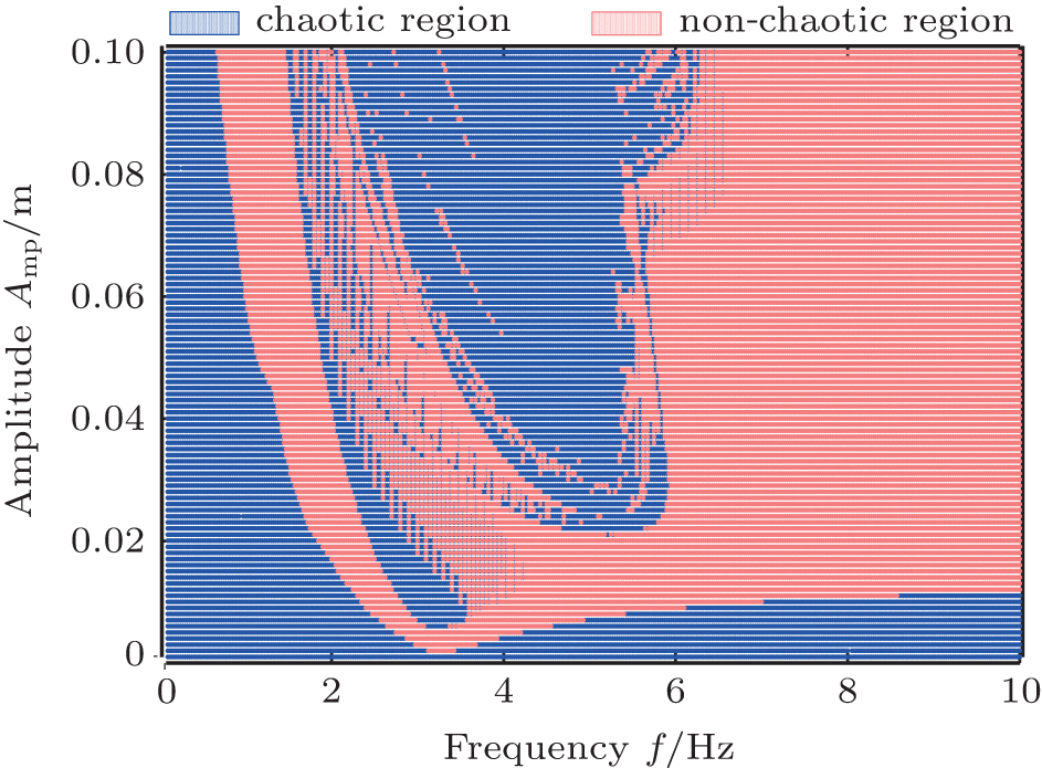 | Fig. 3. Two parameters space plot: frequency versus amplitude of harmonic excitation. |
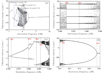
To have better insight into the dynamic evolution process, and to verify the above parameter space plot, the bifurcation diagram under parameter variations is plotted. Figure
 | Fig. 4. Global and partial enlarged bifurcation diagrams versus excitation frequency f, (a) global bifurcation diagram for 1–10 Hz with an increment step of 0.0001, (b) local bifurcation diagram for 2.1–3.2 Hz with an increment step of 0.0001, (c) local bifurcation diagram for 3.365–3.395 Hz with an increment step of 0.00001, (d) local bifurcation diagram for 4.91–5.31 Hz with an increment step of 0.0001. |
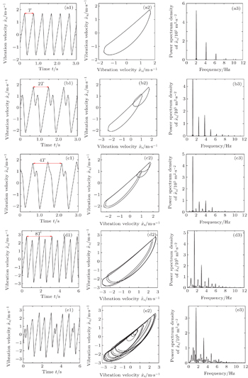
The time histories, phase portraits, and PSD diagrams of the system are depicted, to make a rather intuitive presentation of the dynamical behavior. The dynamical evolutions of the system are presented in Figs.
 | Fig. 5. Time series, phase portraits, and PSD for varying frequencies in the PDB corresponding to Fig. |
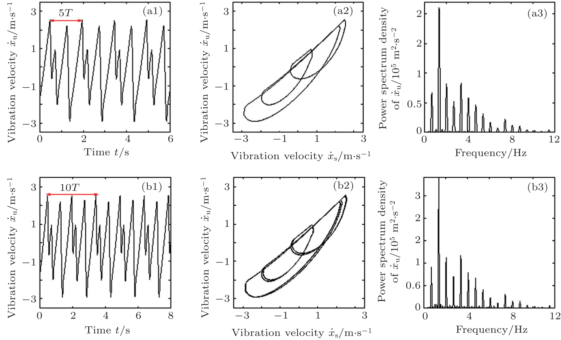 | Fig. 6. Time series, phase portraits, and PSD for varying frequencies in the periodic window of period-5 orbits corresponding to Fig. |
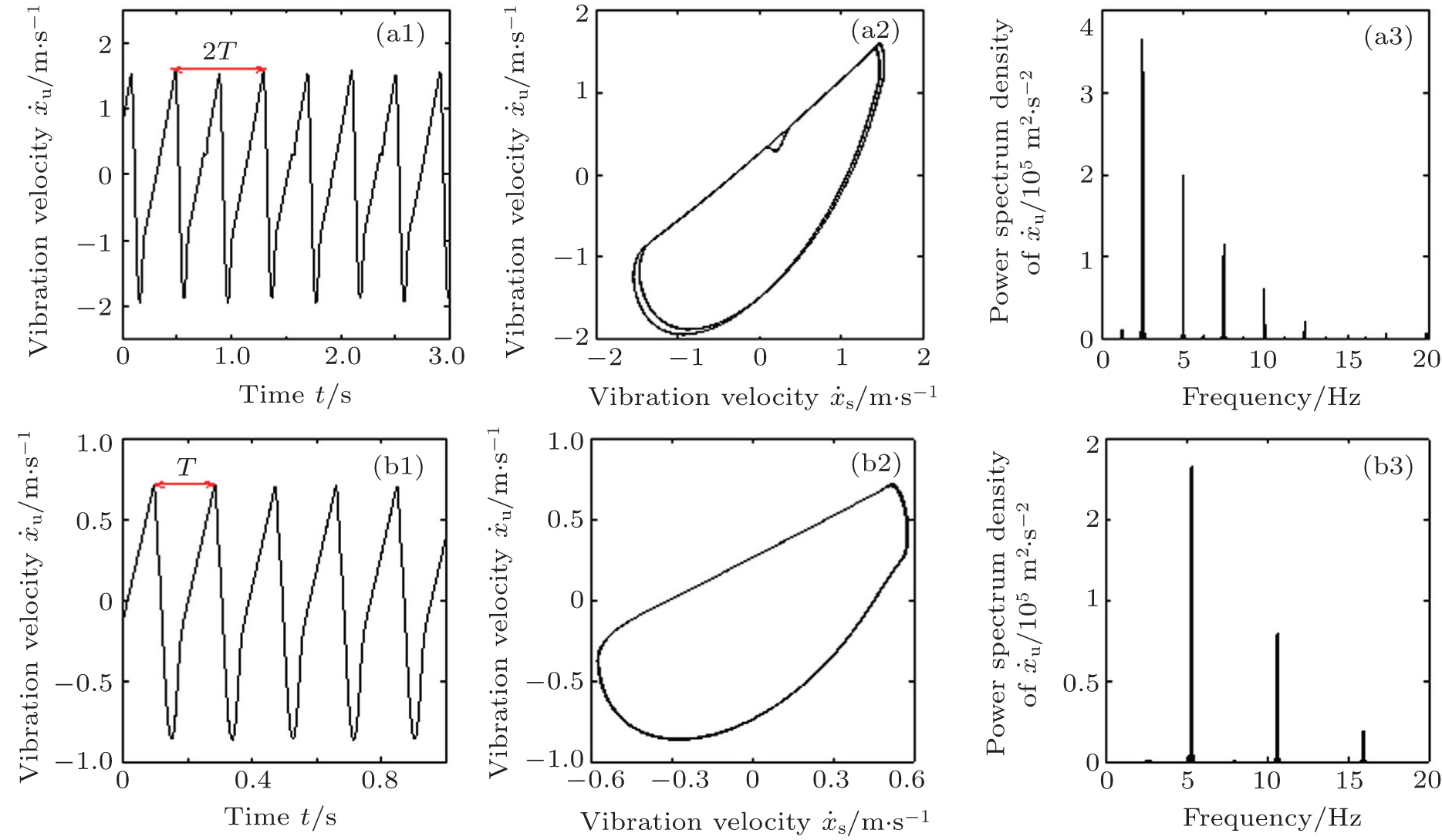 | Fig. 7. Time series, phase portraits, and PSD for varying frequencies in the inverse PDB corresponding to Fig. |
The system escapes from the chaotic region by the SNB, which is shown from the bifurcation diagram in Fig.
Figure
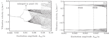
Amplitude is another important parameter of excitation, which plays a critical role in the dynamic responses. Figures
 | Fig. 8. Global and partial enlarged bifurcation diagrams versus the excitation amplitude Amp: (a) global bifurcation diagram for 0.005–0.1 m with an increment step of 0.00001, (b) local bifurcation diagram for 0.041–0.049 m with an increment step of 0.000001. |
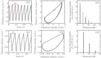
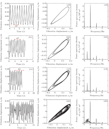
Figure
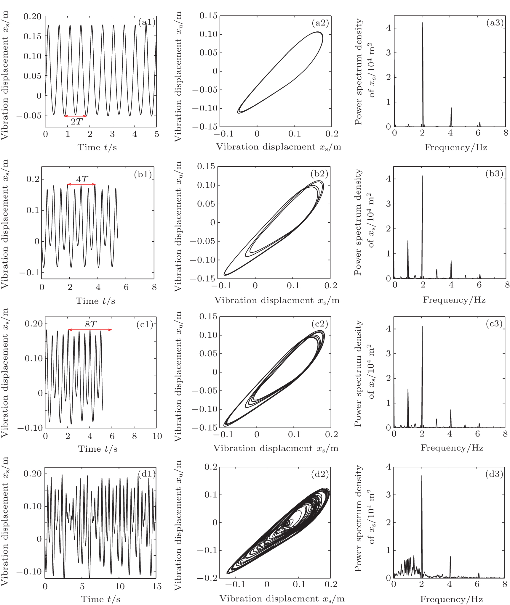 | Fig. 9. Time histories, phase portraits, and PSD for different Amp in the PDB: (a1)–(a3) 0.04372 m, (b1)–(b3) 0.047245 m, (c1)–(c3) 0.04793 m, and (d1)–(d3) 0.0558 m. |
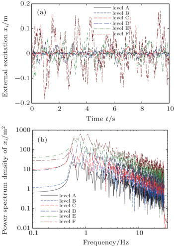
More generally, random excitation is the most common form of external disturbance for the vibration isolation system. Here, the bounded stochastic road spectrum is considered as the external excitation for MR suspension. The spectral density function of the road surface is first defined as follows:


The parameters in this paper are given as: v = 30 km/h, fmin = 0.5 Hz, fmax = 30 Hz, and t = 10 s. The distributed time step is set as 0.0001 to avoid a shortage of storage space, then N is calculated at 100000. The road level is divided into six levels according to the different Gq(f0), and that is, level A corresponding to 16 × 10−6, level B corresponding to 64 × 10−6, level C corresponding to 256 × 10−6, level D corresponding to 1024 × 10−6, level E corresponding to 4096 × 10−6 and level F corresponding to 16384 × 10−6, respectively. Figure
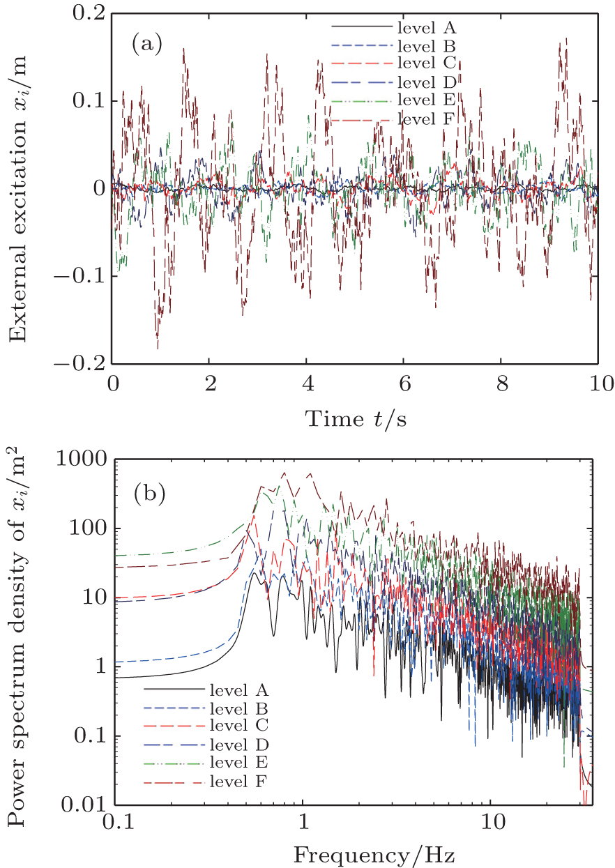 | Fig. 10. Time history (a) and power spectrum density (b) of six levels of excitation. |
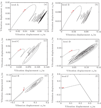
Phase portraits of xs versus xu are plotted in Fig.
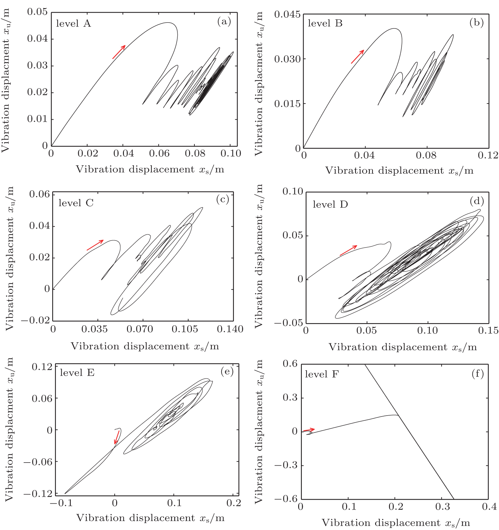 | Fig. 11. Phase portraits of different levels of road surface. Panels (a)–(f) correspond to levels A–F, respectively. |
The LE is used again to determine the chaos. The C–C method is adopted to calculate the embedded dimension and delay time for phase space reconstruction, and after that, the LLEs under the six levels are obtained. Besides, Kolmogorov entropy (K entropy) is the effective evaluation index for distinguishing chaos from stochastic and stable state.[28] Thus, K entropies under the six levels are calculated by using the least square method. As is listed in Table
| Table 1. Largest Lyapunov exponent and K entropy for different levels. . |
These results are complete verification of the set of parameters where chaos may occur in MR suspension system under external excitation. For harmonic excitation, the frequency shows insensitive characteristics of mid-frequency of 3–5 Hz, where the chaotic motions and periodic windows exist alternately. Meanwhile, with the increase of amplitude, chaotic motions appear through the PDB. The threshold value is regular of around 0.03 m, thereby illustrating the great possibility of the appearance of chaotic motions in practical application. The chaotic area we obtained is consistent with that obtained in Ref. [15], which is also the low- and mid-frequency. What is more, the results here are more realistic, especially for the amplitude of chaotic motions, compared with that of exaggerated 0.36 m of the 1-DOF simplified model used in Ref. [18]. As for the random road surface, the larger the PSD of excitation, the more likely chaotic motions will occur in the MR suspension system. As shown in Figs.
The analytic method used in this paper could be generalized to other nonlinear systems. That is, the global chaotic features analysis is first conducted by the two- or three-parameter plot based on LLEs with varying parameters. After that, the typical parameter domain is further studied thoroughly, to demonstrate the process of the nonlinear dynamic evolution. Meanwhile, the bandwidth-limited stochastic excitation used here can be used for nonlinear dynamic analysis on a non-autonomous system with the general external disturbance. Moreover, in this case, the K entropy is an effective and convenient means for distinguishing the chaos from stochastic.
As a note of caution, however, the integrated vehicle MR suspension system consists of four or more 2-DOF sub-systems used in this paper, which means that the dynamic model is with a higher DOF, and the nonlinear dynamic analysis of the system needs to be conducted. Moreover, the MR suspension system usually works with the semi-active mode. To reveal the nonlinear dynamic of semi-active MR suspension is the ultimate goal, while the passive current is used here for basic research.
The nonlinear dynamic responses of an MR suspension system were assessed with the methods of nonlinear dynamics. Various system responses for road parameters change (under the external excitation of harmonic and random road surface), such as time histories, bifurcation diagrams, phase planes, and PSD diagrams were observed using the 2-DOF MR suspension model with modified Bouc–Wen hysteretic MRD model. The result was a range of possible parameters of external excitation, where unstable responses existed. Under a single frequency harmonic excitation, the small amplitude is below about 0.005 m, and the middle-low frequency of 0.1–6 Hz is more likely to cause instability phenomena even chaos. In addition, chaotic motions are more likely to appear when riding through rough road surfaces. While riding through the relatively flat road surface, the vertical vibration of the MR suspension system is restricted within the limited state space. The obtained exact excitation profiles and chaotic regions in the paper may influence semi-active control strategies designed for the MR suspension system. The analysis may contribute to reliably implementing MRD to structural vibration semi-active control systems, and to researching the smart materials with hysteresis phenomenon and nonlinear characteristics. In the subsequent work, research on chaotic suppression and hardware experiments will be conducted.
| 1 | |
| 2 | |
| 3 | |
| 4 | |
| 5 | |
| 6 | |
| 7 | |
| 8 | |
| 9 | |
| 10 | |
| 11 | |
| 12 | |
| 13 | |
| 14 | |
| 15 | |
| 16 | |
| 17 | |
| 18 | |
| 19 | |
| 20 | |
| 21 | |
| 22 | |
| 23 | |
| 24 | |
| 25 | |
| 26 | |
| 27 | |
| 28 |