A quantum phase transition (QPT)^[1,2] is driven by quantum fluctuations in the ground state of a many-body system. As an external parameter such as a magnetic field varies, the qualitative structure of the system's ground-state wavefunction exhibits an abrupt change across the quantum critical point. With this observation, researchers were motivated to use the fidelity, which is a concept borrowed from the quantum information theory, to study QPTs.^[3,4]

Fidelity measures the similarity between two states. Mathematically, the static ground-state fidelity is defined as the magnitude of the overlap between two ground states differing from each other by a small value in the parameter space. Within one phase of the system, the two states have similar structures and thus the fidelity is close to unity. On the other hand, the ground states in distinct phases of the system are significantly different from each other. The fidelity is thus expected to show a sudden drop across the quantum critical point. The significance to use fidelity and its variations, such as fidelity susceptibility,^[5,6] generalized fidelity susceptibility,^[7] fidelity per site,^[8,9] reduced fidelity,^[10,11] operator fidelity,^[12,13] and density-functional fidelity,^[14] as a probe of QPTs have been testified in a number of condensed matter models (for a comprehensive review, please refer to Ref. [15]). Recently, an equality relating the fidelity susceptibility and the spectral function has been derived.^[16] This makes the fidelity susceptibility to be directly measurable in experiments via neutron scattering or the angle-resolved photoemission spectroscopy (ARPES) techniques.

Although the fidelity can well witness a quantum critical point and provide us the critical exponents in continuous phase transitions,^[17–20] the information about the nature and the symmetry of a phase that one could obtain is limited. With the motivation to gain more insight about a quantum phase from the fidelity approach, we proposed the fidelity spectrum in this work. Recently, Gu et al.^[21] and Sacramento et al.^[22] also introduced the concepts of mode fidelity and fidelity spectrum, respectively, with similar motivations.

In Sacramento and his collaborators' proposal, the fidelity spectrum was defined through the fidelity operator where ρ₁ and ρ₂ are the reduced density matrices. The focus was on the partial state of the system. However, the global ground state of the system usually plays a role in a QPT. Especially in a topological QPT in which the global topological order of the system changes,^[23] it may be insufficient to just consider the partial state of the system to characterize the quantum phase. At this point, we were motivated to define the fidelity spectrum using the global ground-state wavefunction of the system. We investigated the distributions of the spectra in the one-dimensional (1D) Ising model in a transverse field and the two-dimensional (2D) Kitaev model on a honeycomb lattice. The spectra were found to exhibit qualitative different behaviors in different regimes of the models. From the distributions of the spectra, one can determine the dominating k modes in a phase.

The paper is organized as follows. In Section 2, we established a general mathematical framework of the fidelity spectrum. The fidelity spectrum was studied in the 1D transverse-field Ising model, which exhibits a continuous QPT, and the honeycomb lattice Kitaev model, which exhibits a topological QPT. The results are discussed in Sections 3 and 4, respectively. Finally, a summary is given in Section 5.

Consider a general form of Hamiltonian,

Consider the overlap

Physically, the fidelity spectrum tells us how much the ground state of the final Hamiltonian comes from different eigenstates of the initial Hamiltonian. When the system is under an external perturbation δλH_I, the perturbed ground state is in general a superposition of the eigenstates of the unperturbed Hamiltonian. The contribution from the ground state is given by the fidelity while the contribution from the n-th excited state of the original Hamiltonian is governed by M_n. As one can see from Eq. (7), the fidelity spectrum depends on the scattering amplitude of the driving Hamiltonian and also the energy gap between the ground state and the excited state. By investigating the distribution of {M_n}, we expect to gain information about the modes that are dominating in a quantum phase.

To have a quantitative description of the distribution of {M_n}, we introduce a quantity

The 1D transverse-field Ising model is one of the simplest many-body systems, which is exactly solvable and exhibits a QPT.^[27–31] The Hamiltonian of the model is given by

The model’s Hamiltonian can be diagonalized through standard procedure using the Jordan–Wigner transformation, Fourier transformation, and Bogoliubov transformation.^[1] After these transformations, equation (9) becomes

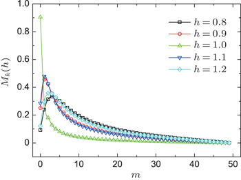
To investigate the fidelity spectrum in Eq. (7), we take the driving Hamiltonian as

Figure 1 shows the distribution of M_k over the k-space for various values of h. From the figure, we see that for h away from the critical point, the distribution of the fidelity spectrum is more widely spread. However, at the critical field h = 1, the distribution is dominated by the zero-th mode and shows an exponential decaying trend away from this mode. One may understand this behavior by referring to Eq. (7) and noting that the energy gap between the ground state and the first excited state vanishes at the critical point.

Fig. 1.

	Figure Option ViewDownloadNew Window
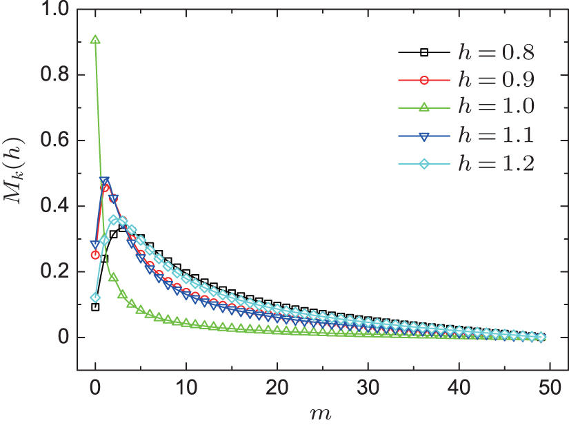
	Fig. 1. A plot of Mk in Eq. (13) distributed over the k-space for the 1D transverse-field Ising model. Here N = 100 and k = (2m + 1)π/N. Only positive k’s are shown.

Quantitatively, we can also obtain the dominating mode by considering dM_k/dk = 0 which gives cosk = 2h/(1 + h²). For h = 1, k = 0 is a solution to the equation. However, note that for N is even, k = (2m + 1)π/N and the k = 0 mode is not allowed in a finite system. Instead, M_k peaks at k = π/N, which in turn tends to zero as N tends to infinity.

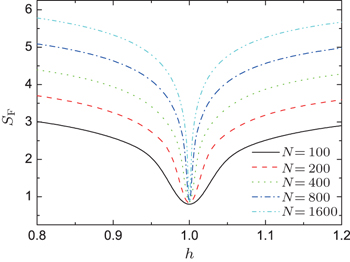
Figure 2 shows a plot of S_F as a function of h for various system sizes. At h = 1, the fidelity spectrum is dominated by the zero-th mode. S_F is thus a minimum as expected. On the other hand, the fidelity spectra in the non-critical region are more spread and S_F becomes larger.

Fig. 2.

	Figure Option ViewDownloadNew Window
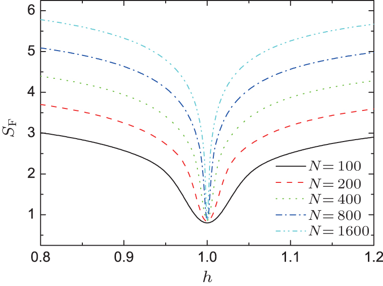
	Fig. 2. SF as a function of h for various system size in the 1D transverse-field Ising model.

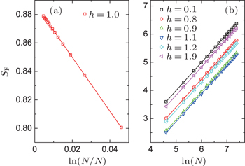
In addition, a point worth noting from the figure is that S_F is insensitive to the system size at the critical point while it shows a non-trivial scaling behavior with N for h ≠ 1. For h = 1, the size dependence of S_F can be obtained analytically. Putting Eq. (13) into Eq. (8), we have

Figure 3 shows a plot of the scaling dependence of S_F with the system size. From linear fitting, we obtain

Fig. 3.

	Figure Option ViewDownloadNew Window
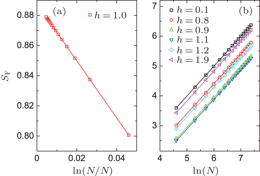
	Fig. 3. (Left) The scaling behavior of SF at the critical point of the 1D transverse-field Ising model. The straight line shows the linear fit of −1.89lnN/N + 0.89. (Right) The scaling behavior of SF in the non-critical region. The slope of the straight line is 1 (maximum error = ±0.001).

The Kitaev model was first introduced by Kitaev to study anyonic statistics.^[36] The ground state of the model can be exactly obtained and it is found to possess a topological QPT.^[36,37] Its ground-state phase diagram consists of gapless phases with non-Abelian anyon excitations and gapped phases with Abelian anyon excitations. As an exactly solvable 2D model exhibiting such an interesting phase diagram, the Kitaev model and its extensions have been intensively studied in the field of condensed matter physics (for examples, please see Refs. [38]–[42]). Besides, the model also captured much attention in the field of quantum information processing for its potential to realize the fault-tolerant quantum computation.^[43]

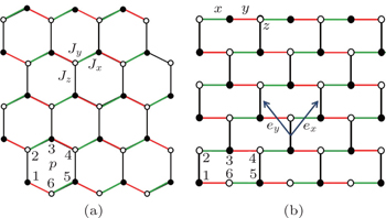
The model consists of 1/2 spins located at the vertices of a honeycomb lattice. They are interacting with the nearest neighbors through three types of bonds, namely, x, y, and z bond, depending on their directions (see Fig. 4). The Hamiltonian reads ^[36]

Fig. 4.

	Figure Option ViewDownloadNew Window
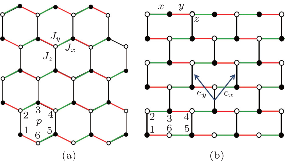
	Fig. 4. (a) A sketch of the Kitaev model on a honeycomb lattice. The lattice can be divided into two equivalent triangular sublattices denoted by the black and white dots. (b) A deformation of the honeycomb lattice on the left into a topologically equivalent brick-wall lattice. ex and ey are the unit vectors connecting the mid-point of the z bonds.

Consider the plaquette labeled as p in Fig. 4. The operator commutes with the Hamiltonian for all p. Obviously, W_p of different plaquettes also commute. Therefore, the Hilbert space can be divided into subspaces with w_p = ±1 for each plaquette. The ground state lies in the subspace in which all w_p are equal to one. This is the key feature that makes an exact solution to the model possible.^[36,37]

The Hamiltonian in Eq. (18) can be diagonalized by two different methods.^[36,37] Following the approach introduced by Chen et al. in Ref. [37], the honeycomb lattice is first deformed into a topologically equivalent brick-wall lattice by stretching the lattice horizontally (see Fig. 4). Defining the Jordan–Wigner transformation as

Introducing the Majorana fermion operators

For

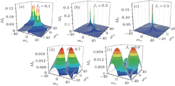
To calculate the ground-state fidelity spectrum, let us consider varying J_z along the J_x = J_y line on the J_x + J_y + J_z = 1 plane (see the red dashed line in the inset of Fig. 6). The interaction Hamiltonian is given by

The distribution of M_k over the k space for J_z = 0.1, 0.3, 0.5, 0.7, 0.9 are shown in the 3D plots in Fig. 5. In the gapless phase where J_z < 0.5, the fidelity spectrum consists of four peaks. These peaks become more concentrated to the zone center as the value of J_z approaches the critical point at J_z = 0.5. While in the gapped phase (J_z > 0.5), the spectrum becomes more dispersive and there is no singular peak.

Fig. 5.

	Figure Option ViewDownloadNew Window
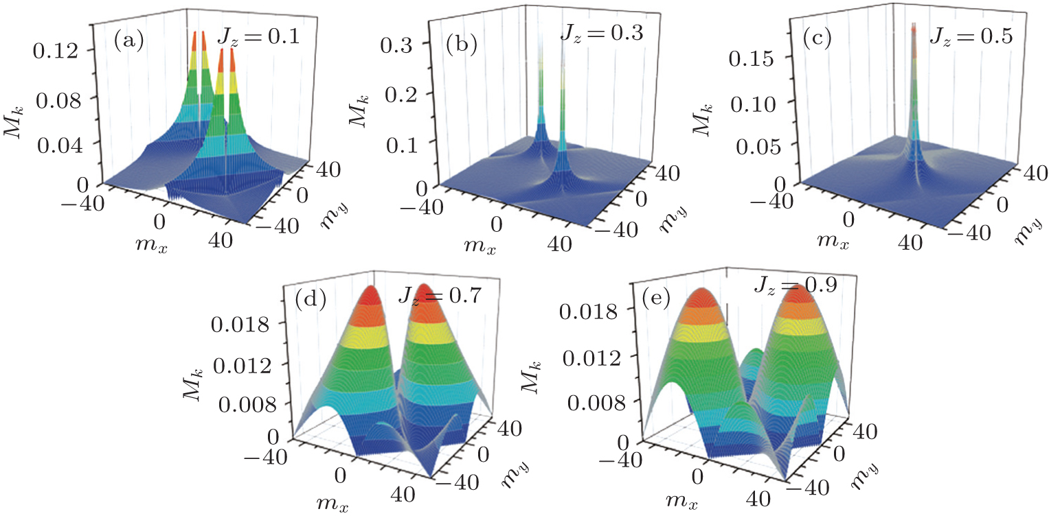
	Fig. 5. 3D plots of the distributions of Mk over the k space for (a) Jz = 0.1, (b) 0.3, (c) 0.5, (d) 0.7, (e) 0.9 in the Kitaev model. Here kx = (2mx + 1)π/L and ky = (2my + 1)π/L, and L = 100.

The behavior of the fidelity spectrum in the gapless phase of the Kitaev model is similar to that at the critical point of the Ising model in which the energy gap vanishes. When the system is gapless in the energy spectrum, the ground state is readily excited to other states. From the peaks in the fidelity spectrum, one can immediately realize which modes’ contributions are the largest for various values of J_z.

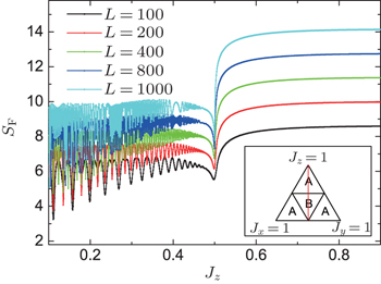
Figure 6 shows a plot of S_F in Eq. (8) as a function of J_z for various system sizes. From the figure, we see that S_F for J_z < 0.5 is smaller than that for J_z > 0.5. This echoes the fact that the fidelity spectrum in the gapless phase is less dispersive than that in the gapped phase.

Fig. 6.

Figure Option ViewDownloadNew Window

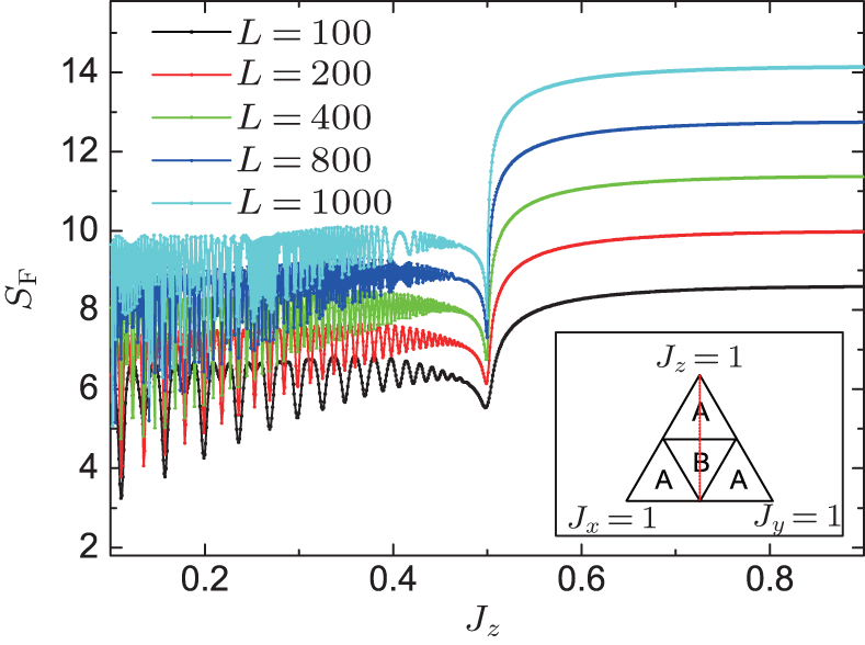
Fig. 6. SF as a function of Jz for various system size. The lines represent the cases for L = 100, 200, 400, 800, and 1600, respectively, when going upward. The inset shows a schematic phase diagram on the Jx + Jy + Jz = 1 plane of the Kitaev model. The A phase is gapped, while the B phase is gapless. A topological QPT takes place at Jz = 0.5 along the Jx = Jy line (as indicated by the dashed line).

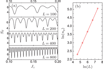
Moreover, S_F in the gapless phase is an oscillating function of J_z. This feature comes from the periodic level-crossing occurred in the excited states of the system. The oscillation patterns are magnified in Fig. 7. As the system size increases, the number of oscillation cycles increases. From the linear fitting on the right panel in Fig. 7, we find that

Fig. 7.

	Figure Option ViewDownloadNew Window
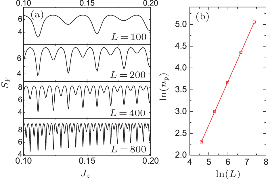
	Fig. 7. (a) Oscillating pattern of SF in the gapless phase. (b) Size dependence of the number of peaks (np) in SF in the gapless phase. The slope of the straight line is 0.991 ± 0.004.

Fig. 8.

	Figure Option ViewDownloadNew Window
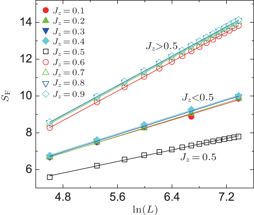
	Fig. 8. Scaling behavior of SF for various values of Jz. The straight lines are the linear fitting of the data points.

Interestingly, like the Ising model, the pre-factor of the size dependence of S_F in the gapped region is also equal to unity. If we express the scaling behaviors in the two models both in terms of N, we have

In summary, we investigated the fidelity spectra in the 1D transverse-field Ising model which exhibits a continuous QPT, and in the 2D honeycomb lattice Kitaev model which exhibits a topological QPT. We found that the fidelity spectrum shows qualitatively different behaviors in different phases of the model. A common feature about the spectrum is that the distribution is dominated by certain k modes in the gapless region while it is more dispersive in the gapped region.

To characterize the distribution of the fidelity spectrum quantitatively, we introduced the quantity S_F in analogy to the Shannon entropy. It was found that at the critical point of the Ising model, S_F ∼ ln N/N while it scales with lnN in the non-critical region. The latter scaling behavior also holds for the Kitaev model. The universality of the relation in Eq. (36) requires further exploration.