Quantum entanglement is considered as a resource of quantum information and computation processing which has no classical analogy^[1–3] and can be only introduced for quantum systems.^[4,5] Quantum entanglement has been used as a useful investigative resource^[6] in quantum teleportation, quantum communication,^[7,8] and quantum computation.^[9]

There have been many studies focused on entanglement at finite temperatures and quantum phase transitions for various spin models such as Ising model, XX model, XY model, XYZ model, XXZ model,^[10–17] isotropic^[18] and anisotropic^[19] Heisenberg spin chain,^[20,21] in the presence^[16,19,22] or absence^[23] of an external magnetic field. Nowadays, the reason for paying attention to the spin models is that they have many established applications in the field of physics such as optical science^[24,25] and entanglement control.^[26]

Lately, researchers are interested in verifying the pairwise entanglement of the Heisenberg model^[17,27] in an equilibrium state at temperature T in the presence of an external magnetic field B. To perform this work, they use some variables for realizing whether systems are entangled or not. For example, concurrence,^[2,15,28] quantum discord,^[11,29,30] entanglement of formation,^[14,31] von Neumann entropies,^[31,32] negativity,^[33,34] and heat capacity.^[35] For scientific reasons, they used some of these quantities to obtain critical points at which phase transitions occur.^[36–38] In addition, from the application aspects, they found some witness operators that are able to detect entanglement for quantum systems.^[39–42]

Pairwise entanglement of mixed-spin systems has been verified in the literature.^[23,43–52] In this paper, we consider a mixed-three-spin cell of a mixed-N-spin chain with Ising–XY model in the presence of an external homogeneous magnetic field B. Its nearest neighbour spins (1,1/2) have Ising-type interaction and the next-nearest neighbour spins (1/2,1/2) have XY-type interaction together. Also, single-ion anisotropy interaction has been considered for spins-1.

One can gain some thermodynamic parameters of a quantum thermal system by means of density matrix ρ as follows:

For instance, heat capacity of the system C^[53] is given by

In this direction, for verifying pairwise entanglement of a bipartite system (qubit–qubit or qubit–qutrit) positive partial transpose criterion (PPT)^[6] was introduced. According to this criterion, if all eigenvalues of the partial transpose of ρ are greater than or equal to zero then, we say that ρ has positive partial transpose (PPT). Therefore, the PPT criterion can be used for introducing a measure of the amount of the distillable entanglement contained in a state. This measure is called negativity, which for the first time was introduced by Vidal and Werner.^[34] Therefore, we use the negativity to investigate pairwise entanglement of the bipartite (sub)system, i.e., the spins (1/2,1/2). For a given density matrix ρ, one can define the negativity as a measure of entanglement based on the amount of violation of the PPT criterion^[33,34] as

By means of the total density matrix of our favorite tripartite system, we extract heat capacity of the system, density matrix, and the negativity for spins (1/2,1/2) as a bipartite (sub)system, which from point of quantum correlation view should be investigated (Section 2). In Section 3, we numerically calculate and simulate the heat capacity of the tripartite system and also, the negativity (as a measure of entanglement^[31]) for investigating pairwise entanglement of the spins (1/2,1/2). Moreover, we introduce some hermitian operators which can be considered as entanglement witnesses for the tripartite system, and finally, some comparisons are done between these witnesses and the heat capacity of the system. Section 5 summarizes our results.

We theoretically introduce the Hamiltonian of the anti-ferromagnetic mixed-spin system with Ising-type and XY-type interactions which is in the external homogeneous magnetic field B as follows:

Hence, we can extract the negativity for the spins (1/2,1/2) and also the heat capacity of the tripartite system, by means of Eq. (10) and the partition function of the system, respectively. Behaviors of these quantities with respect to the temperature, the magnetic field, and anisotropy parameter γ, are presented in the next section.

In this section, we numerically calculate and simulate the heat capacity of the introduced anti-ferromagnetic mixed-three-spin Ising–XY model, and the negativity for the pair spins (1/2,1/2). Heretofore, some interesting results about pairwise entanglement for similar bipartite (sub)systems have been introduced in previous works, for example, in Ref. [43], quantum correlation was investigated by means of the exact calculation of the entropy and the concurrence. We plot some figures to demonstrate and better understand the behaviors of the introduced quantities in this section.

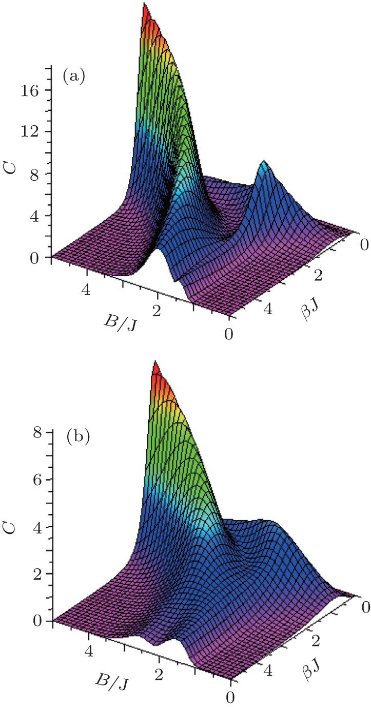
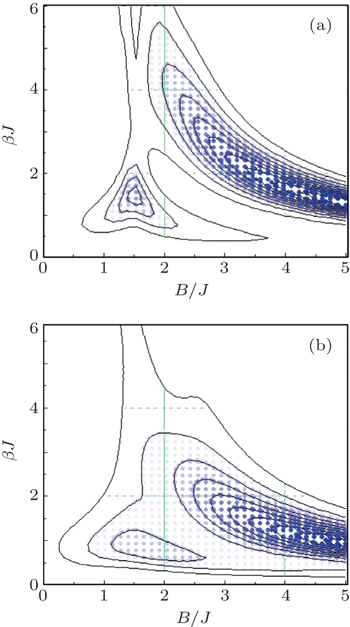
3.1. Heat capacity

Heat capacity as a function of the temperature and the magnetic field at fixed values of the anisotropy parameter γ and single-ion anisotropy coefficient , is shown in Fig. 1. As illustrated in Fig. 1(a), at high temperatures and fixed γ = 0.2J, the heat capacity is maximum at strong magnetic fields. At B ≈ 2J, it also has a smaller separate maximum. By increasing the anisotropy, these two maxima gradually merge (Fig. 1(b)) at fixed values of the temperature T ≈ J and . In addition, by decreasing the temperature at fixed γ = 0.2J (Fig. 1(a)), both of the maxima merge together and will form a single small maximum at finite temperatures.

Fig. 1.

	Figure Option ViewDownloadNew Window
	Fig. 1. Heat capacity of the mixed-three-spin system as a function of the inverse temperature and the magnetic field, at fixed values of and (a) γ = 0.2J; (b) γ = 0.8J.

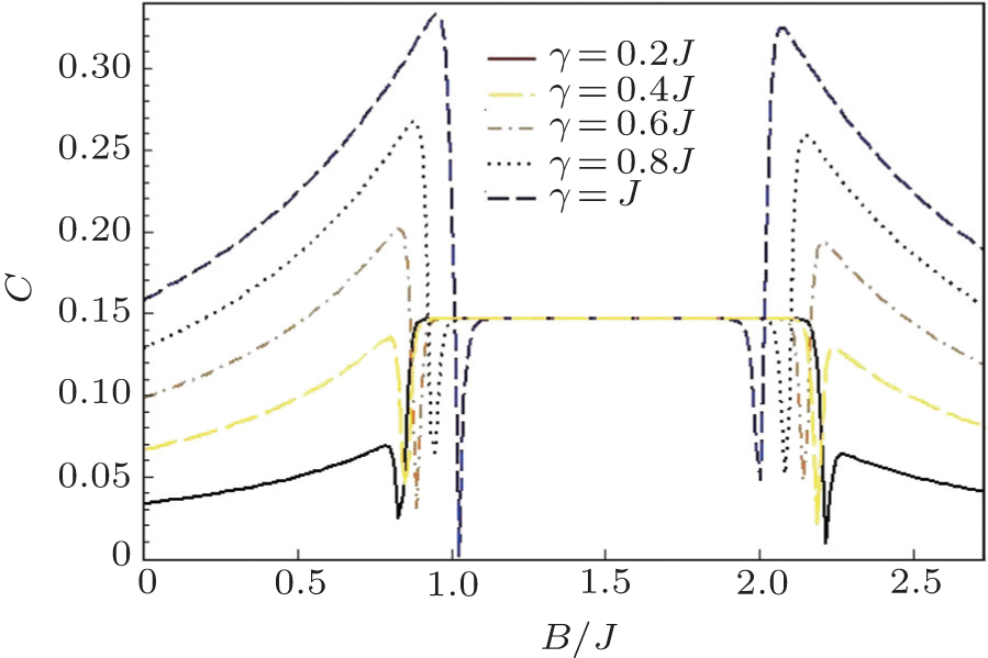
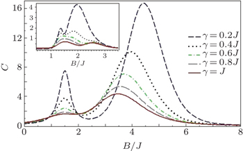
The behavior of these maxima at fixed values of the anisotropy versus the magnetic field is shown in Fig. 2. As shown in this figure, with the increase of the anisotropy, both of the maxima decrease and move towards each other, then merge together and make a single maximum at γ = J. Inset of this figure shows the anisotropy effects on the heat capacity at finite temperatures and fixed value of the single-ion anisotropy coefficient . One can see that, at fixed γ = 0.2J, the heat capacity also has two maxima, where the second maximum (at B ≈ 2J) is greater than the first one. By increasing the anisotropy, the greater maximum gradually decreases and a third maximum arises simultaneously. Finally, with further decreasing the temperature, the second maximum vanishes and just the first and third maxima remain for the heat capacity. Despite all of these, by decreasing the anisotropy, maximum values of the heat capacity decrease up to C < 5 for high temperatures and C < 1 for the finite temperatures. As shown in Fig. 1(b), by increasing the anisotropy versus Ising coupling J, both of the remaining maxima merge together at higher temperatures (T ≈ J) moreover, in this range of the temperature and γ = 0.8J (long-dashed line in Fig. 2), the maximum value of the heat capacity is decreased, (note that here changes of B, T, and γ, have been considered with respect to the Ising coupling J).

Fig. 2.

	Figure Option ViewDownloadNew Window
	Fig. 2. Heat capacity of the system as a function of the magnetic field at fixed values of and T ≈ 1.5J with respect to the various fixed values of the anisotropy. Inset shows the heat capacity function at finite temperatures (T ≈ 0.2J).

Now, we want to explain the behavior of the heat capacity, when the state of the system is a separable state and when it is an entangled state. For weak anisotropy (Fig. 1(a)), at high temperatures and strong magnetic fields when the system is in a separable state, there is a single maximum of the heat capacity. By decreasing the magnetic field, when the system tends to be an entangled state, the second maximum appears, which is smaller than the first one. At the same time, by decreasing the temperature, both of the maxima decrease and move towards each other, and ultimately, merge together and make a single small maximum at fixed B ≈ 2J at finite temperatures (dashed line in the inset of Fig. 2). In the weak magnetic fields B ≪ 2J the heat capacity vanishes, on the other hand (in this range) the system is in an entangled state. In conclusion, shapes of the temperature and the magnetic field dependence of the heat capacity for separable states and entangled states are different. It cannot be possible to comment about the anisotropy dependence of the heat capacity for separable states and entangled states.

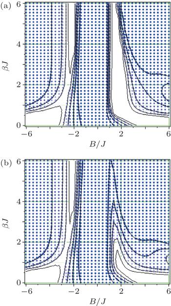
The relationship between the temperature and the magnetic field of the heat capacity function is shown as contour plots of Fig. 1 in Fig. 3. Areas with colored points show the existence of heat capacity (in the range of temperature and magnetic field of these areas, it is estimated that there are some sets of separable states for the tripartite system) and other colorless regions represent the minimum amount of the heat capacity, here, it is estimated that there is at least an entangled state for the tripartite system. Therefore, in a certain interval of the magnetic field, we can consider solid lines of the contour plots as hyper-planes which can separate a convex set of separable states and at least an entangled state outside of this set.

Fig. 3.

	Figure Option ViewDownloadNew Window
	Fig. 3. Contour plots of the heat capacity versus inverse temperature and the magnetic field, at fixed values of and (a) γ = 0.2J; (b) γ = 0.8J.

Hence, if one can find a good relationship between the temperature and the magnetic field at fixed values of the anisotropy and single-ion anisotropy coefficient, then he (or she) can be able to consider each available line of the contour plots of the heat capacity function as an entanglement witness for the tripartite system just as Furman et al. stated in Ref. [53], where they explicitly expressed that if the relationship between the temperature and the magnetic field of the heat capacity function is found, one can introduce it as an entanglement witness. Furthermore, with the increase of the anisotropy, the state of the system tends to be an entangled state and the shape of the heat capacity is here changed simultaneously. This change is visible in Fig. 3 with the change of the solid-line shapes.

These statements for the heat capacity behavior and quantum entanglement of the system are not in general investigative for all quantum systems, just in some special cases it can be effective.

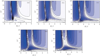
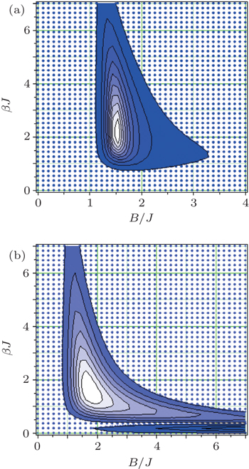
3.2. Negativity

Contour plots of the negativity for spins (1/2,1/2) as a function of the temperature and the magnetic field at fixed values of the anisotropy parameter γ and single-ion anisotropy coefficient , are shown in Fig. 4. By increasing the anisotropy, the shape of the contour plot of the negativity changes; we depict this phenomenon in Fig. 4. In the colorful regions, the negativity is maximum, and at the colorless ones it is minimum. Thereby, we can verify negativity behavior from the color change of its contour plots (colorful regions represent the existence of the negativity). In Fig. 4(a), at high temperatures and weak magnetic fields, the negativity for spins (1/2,1/2) is minimum. By increasing the magnetic field and decreasing the temperature, the negativity appears. With further increasing the magnetic field, the negativity gradually vanishes, and then arises again at B ≈ 1.5J and reaches to maximum amount of itself at B ≈ 2J.

Fig. 4.

	Figure Option ViewDownloadNew Window
	Fig. 4. Contour plots of the negativity as a function of the temperature and the magnetic field at fixed values of and (a) γ = 0.2J; (b) γ = 0.4J; (c) γ = 0.6J; (d) γ = 0.8J; (e) γ = J, for spins (1/2,1/2).

As illustrated in Fig. 4(b), by increasing the anisotropy, colorful regions are expanded, while at the same time, colorless regions (separability) are restricted. With further increment of the anisotropy, the presence of the negativity gradually increases with respect to the temperature and the magnetic field changes (Figs. 4(c) and 4(d)). It is clear that, at high temperatures, the existence of the negativity for strong anisotropy, is more than for weak one. Such as, in the range of the temperature 0 < βJ < 2, by increasing the anisotropy from γ = 0.2J to γ = J, the negativity increases in the interval of J < B < 4J.

Since the negativity is a measure of entanglement, we can verify anisotropy effect on the pairwise entanglement for the spins (1/2,1/2) by means of the anisotropy dependence of the negativity. Therefore, the intensity of the pairwise entanglement with respect to the magnetic field and the temperature is proportional to the increase of the anisotropy. Namely, by increasing the anisotropy, we observe the presence of the pairwise entanglement increasing. As a result, by increasing the anisotropy, the maximum presence of the pairwise entanglement in one region (βJ > 2 and 1.5J < B < 2.5J) in Fig. 4(a), turns into three regions (βJ > 2 and B < J, βJ < 2 and 1.5J < B < 2.5J, βJ < 2 and 2.5J < B) in Fig. 4(e).

We show the negativity as a function of the magnetic field B at finite temperatures, for fixed with respect to the various fixed values of the anisotropy in Fig. 5. By inspecting this figure, one can observe that in the interval of 0 < B < J with the anisotropy decreasing, the peak of the negativity diagram decreases and tends to weaker magnetic fields and gradually approaches to point B = (9 + γ²)/12 that interestingly is a critical point for the mixed-three-spin system in which a quantum phase transition occurs; note that this point is dependent on the anisotropy parameter γ. This peak represents a critical point in which magnetic field phase transition occurs at the finite temperatures for the spins (1/2,1/2).

Fig. 5.

	Figure Option ViewDownloadNew Window
	Fig. 5. The negativity as a function of the magnetic field B at finite temperatures (T = 0.1J) and fixed with respect to various fixed values of the anisotropy parameter γ for spins (1/2,1/2).

In the interval of 1 < B < 2, the negativity is invariant for various fixed values of γ. In this interval of the field, a quantum phase transition occurs for the mixed-three-spin system independent of γ. In the interval of 2 < B < 3, the second peak decreases but tends to the stronger magnetic fields with the anisotropy decreasing, this point is also a critical point in which a phase transition occurs for spins (1/2,1/2). This means that, at finite temperatures, we find an interval of the magnetic field from negativity diagram of a bipartite (sub)system (the spins (1/2,1/2)) of a larger tripartite system (the mixed-three-spin (1/2,1,1/2) system), in which a quantum phase transition occurs for the tripartite system independent of the anisotropy.

Heretofore, Werlang et al. in Ref. [11] for a bipartite quantum system, obviously proved that the quantum discord behavior can present critical points associated with the quantum phase transitions even at finite temperatures.

Now, we introduce as the Hamiltonian of the unperturbed system, whose solutions are well-known. We are interested in investigating the time-independent perturbed system with Hamiltonian

Dowling et al. established Hamiltonians as entanglement witnesses in Ref. [42]. They intelligently suggested entanglement gap category as G_ent = E_sep − E₀, namely, according to their suggestion, the entanglement gap is the energy gap between the ground state energy and the minimum energy that a separable state can access. In addition, they introduced entanglement gap temperature category as well.

In this paper, we expand these definitions and introduce some operators, whose eigenvalues are the first and second-order perturbation corrections to the ground state eigenenergies, as good entanglement witnesses for the introduced Hamiltonian (4).

If we consider the separable state ρ_sep(AB) and the entangled state ρ_ent(AB) which act on Hilbert space H_A ⊗ H_B, then an entanglement witness (EW) is a hermitian operator such that for all separable states, and , which represents the existence of at least an entangled state.

Now, we look quickly at the system from the point of view of the perturbation theory, namely, we introduce the unperturbed system with Hamiltonian as the below equation:

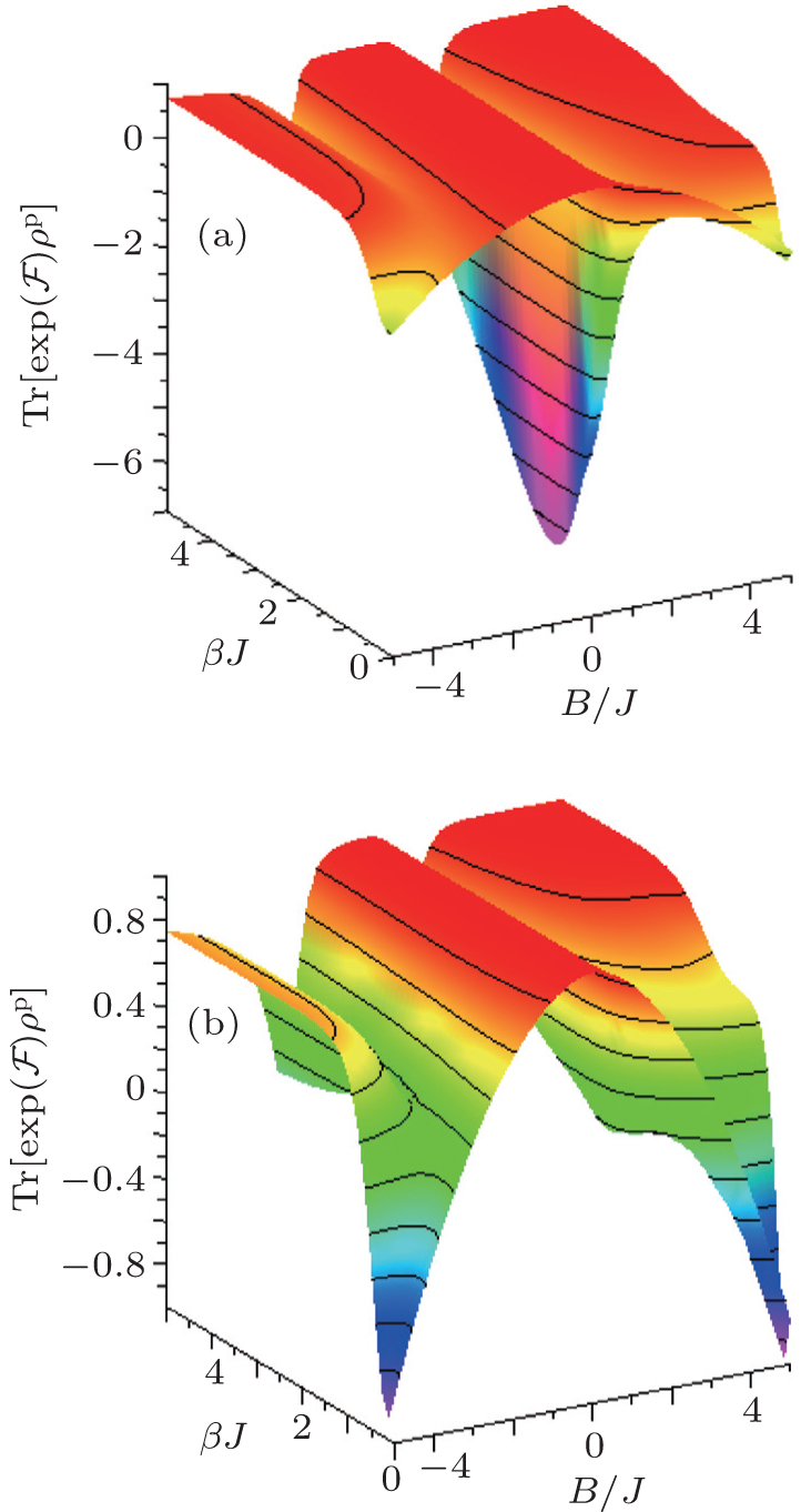
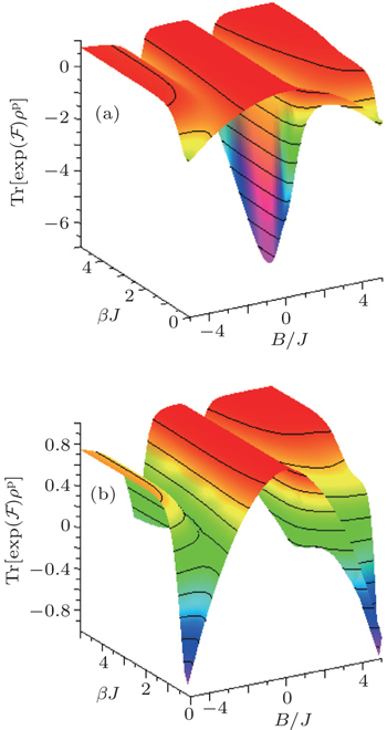
With regard to Eq. (21), the operator is a non-diagonal hermitian matrix, whose product in the perturbed density matrix ρ^p is a non-diagonal matrix therefore , while (and its higher even-powers) product in the density matrix ρ^p has some diagonal elements, therefore, . It is then by addition of this term we can be able to discuss the existence of an operator whose witnesses are at least an entangled state outside of a convex set of separable states for the first-order perturbation correction of Eq. (4). For better understanding, we have numerically calculated and simulated Eqs. (32) and (33) and have presented our results by plotting Fig. 6. As shown in this figure, one can see that in the finite temperatures and weak magnetic fields, equation (32) is established, i.e., cannot be negative. However, by increasing the magnetic field B some points can be found which are less than zero, then equation (33) will be established.

Fig. 6.

	Figure Option ViewDownloadNew Window
	Fig. 6. Detecting entangled states by means of equation (32) at fixed values of and (a) γ = 0.2J, (b) γ = 0.8J.

With regard to Eq. (24), the operator is also a non-diagonal hermitian matrix and, its product in the total density matrix ρ^p is a non-diagonal matrix. does not commute with namely, , so there are some non-zero diagonal elements for matrix . This interesting feature of the hermitian operator makes it different from the hermitian operator (and also its even-powers), and we would like to investigate this mysterious operator, and then describe some novel and worthy of expression outcomes.

By numerically investigating and then simulating and as shown in Figs. 6–8, we realized that these functions have a different behavior for a convex set of separable states and at least an entangled state, namely for the perturbed system, for a set of separable states, we have

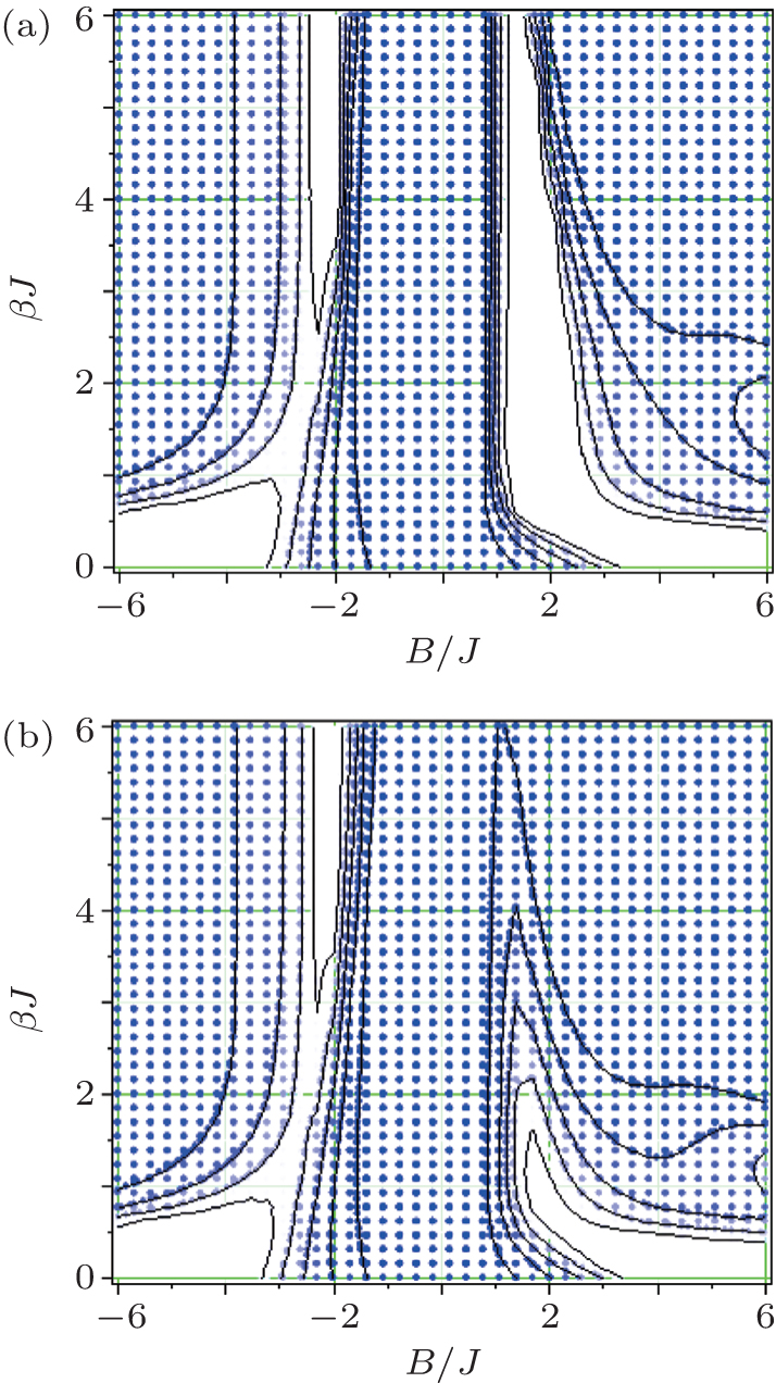
As illustrated in Fig. 7, one can see some hyper-planes (solid-lines) that separate obviously regions containing entangled states (colorless regions) from convex sets of separable states (regions of points). It is clear that, by increasing the anisotropy, some of the hyper-planes vanish, i.e., at finite temperatures and 0 < B < 2 solid-lines gradually disappear. As shown in Figs. 7 and 8, one can see that in the positive values of the field, by increasing the anisotropy, perspicuity of for witnessing entangled states decreases while, the perspicuity of increases, thereby, in the strong anisotropy case, operator witnesses entanglement better than but on the contrary, in the weak anisotropy and also inverse (negative) magnetic fields, operator is a good entanglement witness.

Fig. 7.

	Figure Option ViewDownloadNew Window
	Fig. 7. Contour plots of Fig. 6 versus the inverse temperature and the magnetic field, at fixed values of and (a) γ = 0.2J; (b) γ = 0.8J.

Fig. 8.

	Figure Option ViewDownloadNew Window
	Fig. 8. Contour plots of the function versus inverse temperature and the magnetic field, at fixed values of and (a) γ = 0.2J; (b) γ = 0.8J.

In this work, we first illustrated the heat capacity for the introduced system with Hamiltonian (4), then the negativity for spins (1/2,1/2) has been demonstrated by using its contour plots as shown in Fig. 4. Now, we want to explain an interesting and unusual relationship between these functions and functions and , by comparing Figs. 7 and 8 with Figs. 3 and 4, which represent advantages of the aforesaid operators. As shown in Fig. 3(a), at finite temperatures (T ≪ J) in the interval of 1 < B < 2 the heat capacity vanishes (colorless small region) whose contour plot shows it precisely; on the other hand, in this region, there is at least an entangled state for the tripartite system.

In addition, with regard to Figs. 7(a) and 8(a), we see that, in this interval of the field at finite temperatures, and can be less than zero, namely, both witness some entangled states. These phenomena are consistent with heat capacity vanishing. It is clearly seen that lines in the contour plots of functions and (as hyper-planes with respect to the inverse temperature and the magnetic field) separate convex sets of separable states from entangled states better than ones in the contour plot of the heat capacity, and at high temperatures, operator would be more helpful for detecting entanglement. In addition, for inverse magnetic field this operator is superior yet.

With regard to Fig. 8(b), in the considered interval of the magnetic field 1 < B < 2 and fixed values of and γ = 0.8J, at finite temperatures, lines in the contour plot of are the best hyper-planes which separate the convex set of separable states and some entangled states; therefore, in this condition, operator is a good entanglement witness. In the high temperatures, this operator becomes predominant again for witnessing entanglement.

From Fig. 8 it is clear that, by decreasing the anisotropy from one to zero, at high temperatures, some hyper-planes disappear. Therefore, for weak anisotropy (γ ≪ 1), operator is more useful for witnessing entanglement, and in the stronger anisotropy (γ ≈ 1) operator is a good entanglement witness. Generally, our another aim from these comparisons is that we qualitatively showed that the relationship between temperature and the magnetic field of the heat capacity for our considered system, cannot witness entanglement as well as that one for the introduced traces and in this paper.

In summary, we theoretically investigated the heat capacity behavior of a mixed-three-spin (1/2,1,1/2) Ising–XY model with the nearest-neighbor and that of the next-nearest-neighbour interactions, with respect to the temperature, the magnetic field, and in particular the anisotropy parameter, when the considered system is in a separable state (high temperatures and strong magnetic fields) and when it is in an entangled state (finite temperatures).

In the finite temperatures and weak magnetic fields where the state of the system is an entangled state, we concluded that in these conditions, the heat capacity is minimum. By increasing the temperature and the magnetic field, the state of the system tends to a separable state; in this condition the heat capacity increases from zero to some maxima until it reaches the maximum amount of itself at high temperatures and strong magnetic fields. The behavior of the heat capacity is highly sensitive with respect to the anisotropy changes, namely, with the increase of the anisotropy, peaks of the heat capacity diagram decrease and merge together, on the other hand, the state of the system tends to be an entangled state. In the present paper, it was shown that the behavior of the heat capacity with respect to the anisotropy for separable states is different from entangled states. Moreover, the heat capacity behavior of the system with respect to the temperature and the magnetic field at fixed values of the anisotropy is different between separable states and entangled states, where by increasing the anisotropy, this difference is monotonically reduced. However, it should be noted that these suggestions have been limited to the mixed-three-spin system, and for other systems, in particular the systems with larger number of spins, it is statistically complex and harder to verify the entanglement of such systems.

Thermal pairwise entanglement of the spins (1/2,1/2) has been investigated by calculating and simulating the negativity as a function of the temperature and the magnetic field at fixed values of the anisotropy, also, it has been verified at finite temperatures with respect to the magnetic field, and we presented an interval of the magnetic field in the negativity diagram in which the negativity of the introduced bipartite (sub)system (spins (1/2,1/2)) does not change for various fixed values of the anisotropy parameter, interestingly at this interval, a quantum phase transition occurs for the tripartite spin system (mixed-three-spin(1/2,1,1/2) system).

Therefore, we here showed that at finite temperatures and independent of the anisotropy changes, one is able to determine an interval of the magnetic field in which a quantum phase transition occurs for the tripartite system, by means of the negativity of its bipartite (sub)system (spins (1/2,1/2)) as a function of the magnetic field. In addition, at finite temperatures, some peaks can be seen in which magnetic phase transitions occur, and these critical magnetic fields change with changes of the anisotropy. As was illustrated, in the interval of 0 < B < 1, by decreasing the anisotropy, the peak of the negativity function decreases and moves towards weaker fixed magnetic field B ≈ 0.75 at which a quantum phase transition occurs for the tripartite system (this suggestion can be precisely proved from Eq. (9)). Since, investigating a quantum system in the absolute zero temperature and detecting critical points is very difficult and expensive, in this work we proved that one can detect some critical points in which quantum phase transition occurs for such a system, by investigating the negativity of its (sub)system at finite low temperatures.

We also verified our favorite system from the point of view of the time-independent perturbation theory (non-degenerate case has been considered). In this way, we obtained some operators by using the Dalgarno and Lewis method and then, introduced some interesting entanglement witnesses. Finally, we compared these entanglement witnesses with each other and concluded that, for various ranges of the anisotropy, one of these operators acts better than another one for witnessing entanglement. Moreover, in the present paper, we generally concluded that the relationship between the temperature and the magnetic field of and witnesses entanglement better than one for the heat capacity function C. Investigating this model with other interactions like Dzyaloshinskii–Moriya interaction, in the presence of an external inhomogeneous magnetic field will be attractive to define some new outcomes.