Guner Ozkan, Bekir Ahmet. Bright and dark soliton solutions for some nonlinear fractional differential equations. Chinese Physics B, 2016, 25(3): 030203
Permissions
Bright and dark soliton solutions for some nonlinear fractional differential equations
Guner Ozkan1, †, , Bekir Ahmet2, ‡,
Cankiri Karatekin University, Faculty of Economics and Administrative Sciences, Department of International Trade, Cankiri, Turkey
Eskisehir Osmangazi University, Art-Science Faculty, Department of Mathematics-Computer, Eskisehir, Turkey
In this work, we propose a new approach, namely ansatz method, for solving fractional differential equations based on a fractional complex transform and apply it to the nonlinear partial space–time fractional modified Benjamin–Bona–Mahoney (mBBM) equation, the time fractional mKdV equation and the nonlinear fractional Zoomeron equation which gives rise to some new exact solutions. The physical parameters in the soliton solutions: amplitude, inverse width, free parameters and velocity are obtained as functions of the dependent model coefficients. This method is suitable and more powerful for solving other kinds of nonlinear fractional PDEs arising in mathematical physics. Since the fractional derivatives are described in the modified Riemann–Liouville sense.
The theory of solitons is a fundamental area of research in ocean dynamics and engineering. In this area, the study of solitary waves attracts a lot of attention. Therefore, it is important to focus on solitary waves in a detailed manner from a mathematical point of view. In recent years, nonlinear fractional differential equations (NFDE) have gained importance and popularity in different research areas and engineering applications.[1,2] These equations are used to describe the propagation of long waves in shallow water and also arise in other physical applications such as nonlinear lattice waves, iron sound waves in a plasma, and in vibrations in a nonlinear string. The construction of exact and analytical travelling wave solutions of nonlinear fractional differential equations is one of the most important and essential tasks in nonlinear science and ocean engineering, as these solutions describe very well the various natural phenomena, such as vibrations, solitons, and propagation with a finite speed.
Many reliable methods are used in the solitary waves theory to investigate solitons, and in particular 1-soliton solutions of nonlinear fractional differential equations which appeared in open literature, such as the (G′/G)-expansion method,[3,4] the first integral method,[5] the fractional sub-equation method,[6,7] the exp-function method,[8,9] the fractional functional variable method,[10,11] the fractional modified trial equation method,[12] and so on.[13]
In this work, we convert fractional differential equations into integer-order ordinary differential equations by fractional complex transformation and then we obtain a variety of exact solutions to determine soliton solutions, dark soliton solutions, and bright soliton solutions.[14,15]
There are several approaches to the generalization of the notion of differentiation of fractional orders, e.g., Riemann–Liouville, Grünwald–Letnikow and Caputo.[16,17] Jumarie proposed a modified Riemann–Liouville derivative.[18]
Now, we give some properties and definitions of the modified Riemann–Liouville derivative which will be used in the sequel of the work.
Assume that f : R → R, x → f (x) denote a continuous (but not necessarily differentiable) function. In Ref. [19], Jumarie modified Riemann–Liouville derivative of order α which is defined by
where Γ(x) is the Gamma function. To summarize a few properties of the fractional modified Riemann–Liouville derivative, we give the following three famous formulas:
where a and b are constant.
We consider the following general nonlinear FDE of the type:
where u is an unknown function, and P is a polynomial of u and its partial fractional derivatives, in which the highest order derivatives and the nonlinear terms are involved.
By using the traveling wave variable
where k and c are non-zero arbitrary constants, and by using the chain rule
where and are called the sigma indexes see Refs. [20]–[22], without loss of generality, we can take where l is a constant.
Substituting Eq. (6) with Eqs. (2) and (7) into Eq. (5), we can rewrite Eq. (5) in the following nonlinear ODE:
where the prime denotes the derivation with respect to ξ. If possible, we should integrate Eq. (8) term by term one or more times.
2. The space–time fractional mBBM equation
We consider the following space–time fractional mBBM equation
where v is a nonzero positive constant. This equation was first derived to describe an approximation for surface long waves in nonlinear dispersive media. It also characterizes the hydromagnetic waves in cold plasma, acoustic waves in inharmonic crystals and acoustic gravity waves in compressible fluids. Alzaidy, obtained three types of exact analytical solutions of Eq. (9) using sub-equation method in Ref. [23]. Misirli and Ege, have obtained many analytical exact solutions of this equation with the modified Kudryashov method in Ref. [24]. Bekir et al. have applied the first integral method to obtain new exact solutions of Eq. (9) in Ref. [25]. When α = 1, Eq. (9) is called the modified BBM equation. The modified BBM equation is used in many physical applications. Existence of the solutions for this equation has been considered in several papers, see Refs. [26]–[30]. The bright and dark soliton solutions to Eq. (9) will be obtained by ansatz method.[31–33] For this, we use the following transformations:
where k and λ are nonzero constants. Substituting Eq. (10) with Eqs. (2) and (7) in Eq. (9), we have
where U′ = dU/dξ. By once integrating and setting the constants of integration to zero, we obtain
2.1. The bright soliton solution
The solitary wave ansatz for the bright soliton solution, the hypothesis is[34–37]
where
Here, A, λ, and k are nonzero constants. The unknown p will be determined during the course of derivation of the solutions of Eq. (9). Therefore, from Eqs. (13) and (14), it is possible to obtain
Thus, substituting the ansatz (13)–(16) into Eq. (12) yields
Now, from Eq. (17), equating the exponents p + 2 and 3p leads to
so that
From Eq. (17), setting the coefficients of sechp+2ξ and sech3pξ terms to zero, we obtain
by using Eq. (19) and after some calculations, we have
We find, from setting the coefficients of sechpξ terms in Eq. (17) to zero
also we obtain
From Eq. (21), it is important to note that
Thus finally, the 1-soliton solution of Eq. (9) is given by
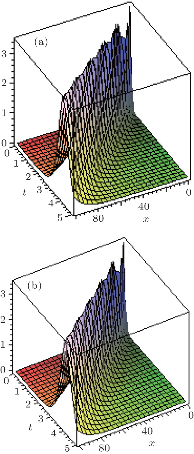
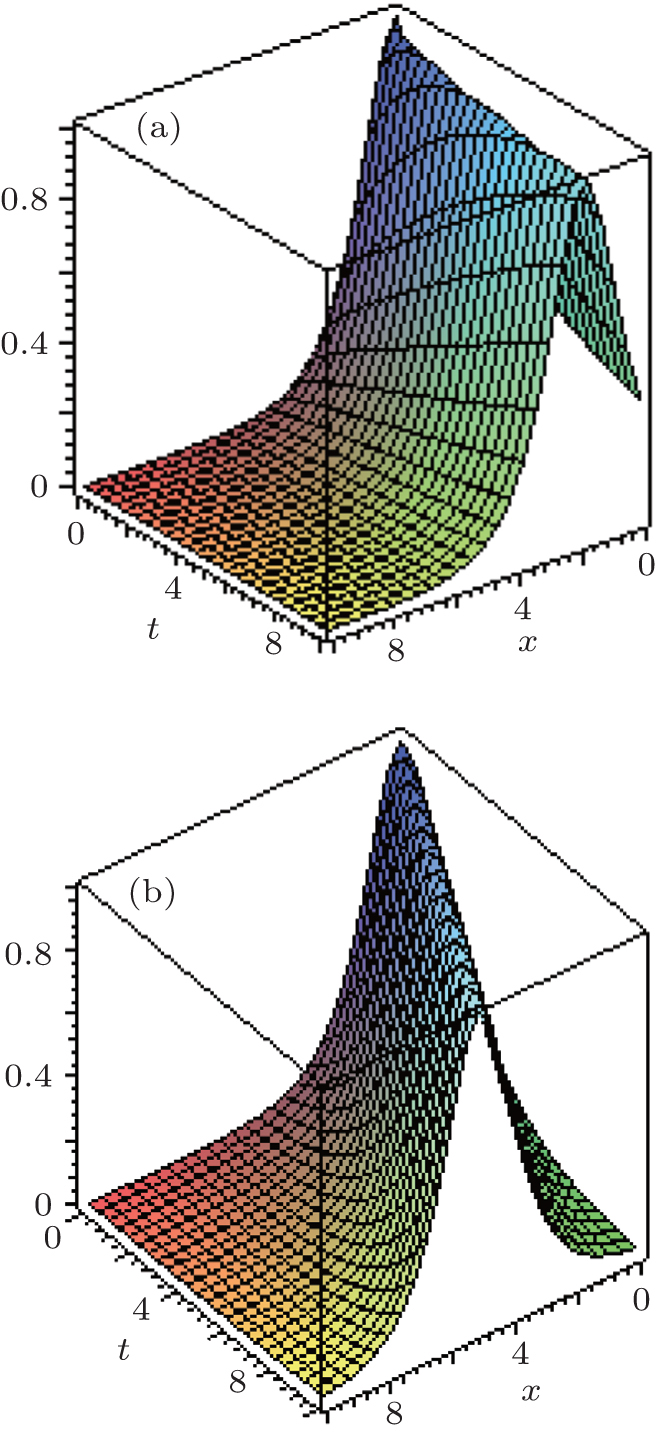
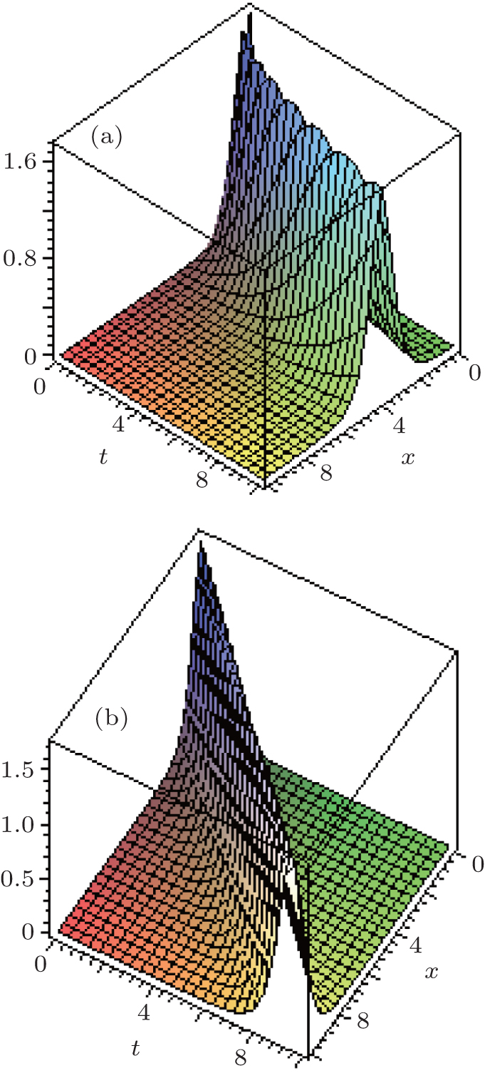
The evolution of exact solution for Eq. (25) with α = 0.5 and α = 1.0 is shown in Fig. 1.
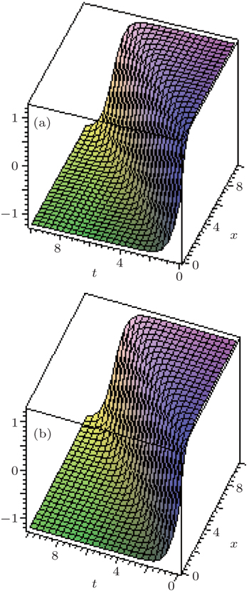
Fig. 2. The exact solution for Eq. (38) with α = 0.5 (a) and α = 1 (b) respectively, when k = 1/2 and v = 1.
3. The time fractional mKdV equation
We consider the following fractional time fractional mKdV equation:[40]
where γ and β are arbitrary constants, α is a parameter describing the order of the fractional time-derivative. The bright soliton solutions to Eq. (39) will be obtained by ansatz method. In order to solve Eq. (39), we use the following transformations:
where k and λ are nonzero constants. Substituting Eq. (40) with Eqs. (2) and (7) in Eq. (39), we have
where U′ = dU/dξ. By once integrating and setting the constants of integration to zero, we obtain
3.1. The bright soliton solution
To obtain the bright soliton solution of Eq. (42), the solitary wave ansatz admits the use of the assumption
where
in which k, λ, and A are constant coefficients. The exponents p is unknown at this point and will be determined later. From the ansatz (43) and (44), we obtain
Thus, substituting the ansatz (43)–(46) into Eq. (42) yields to
Now, from Eq. (47), equating the exponents p + 2 and 3p leads to
From Eq. (47), setting the coefficients of sechp+2ξ and sech3pξ terms to zero, we obtain
by using Eq. (48) and after some calculations, we obtain
We find, from setting the coefficients of sechpξ terms in Eq. (47) to zero
also we obtain
Thus finally, the 1-soliton solution of Eq. (39) is given by
In addition from Eq. (50), it is important to note that γβ > 0. The exact solution obtained is described in Fig. 3.
Fig. 4. The exact solution for Eq. (64) with α = 0.5 (a) and α = 1 (b) respectively, when k = 1, γ = −6, and β = 1.
4. The nonlinear fractional Zoomeron equation
The last equation is called the nonlinear fractional Zoomeron equation which has the form[41]
where u(x,y,t) is the amplitude of the relevant wave mode. In the literature, there are few articles about this equation. Zayed and Amer applied the first integral method to this equation and obtained the hyperbolic, trigonometric, and rational function solutions. Zayed and Arnous obtained periodic, soliton, kink-shaped soliton solutions to the nonlinear fractional Zoomeron equation by means of (G′/G)-expansion method in Ref. [42]. Guner and his colleagues implemented the exp-function method and obtained new exact solutions.[43] When α = 1, the fractional equation reduces to the (2+1)-dimensional Zoomeron equation. We know that this equation was introduced by Calogero and Degasperis. Some of the analytical methods have been proposed for solving this equation (see Refs. [44]–[47] and the references therein).
For our purpose, we introduce the following transformations:
where l, c, and w are non-zero constants. Substituting Eq. (67) with Eqs. (2) and (7) in Eq. (65), we have the ODE
where U′ = dU/dξ. Integrating Eq. (68) twice with respect to ξ, we obtain
where k is a nonzero constant of integration, while the second constant of integration is vanishing.
4.1. The bright soliton solution
To obtain the bright soliton solution of Eq. (69), the solitary wave ansatz admits the use of the following assumption:
where
in which l, c, w, and A are constant coefficients. The exponents p is unknown at this point and will be determined later. From the ansatz Eqs. (70) and (71), we obtain
Thus, substituting the ansatz Eqs. (70)–(73) into Eq. (69), leads to
Now, from Eq. (74), equating the exponents p + 2 and 3p yields
From Eq. (74), setting the coefficients of sechp+2ξ and sech3pξ terms to zero, we obtain
by using Eq. (76), we obtain
so that the solitons will exist for
We find, from setting the coefficients of sechpξ terms in Eq. (74) to zero
also we obtain
which shows that solitons will exist for
Thus finally, the 1-soliton solution of Eq. (65) is given by
where w is given in Eq. (80) and A is given in Eq. (77). The graphs are given in Fig. 5.
Fig. 5. The exact solution for Eq. (82) with α = 0.5 (a) and α = 1 (b) respectively, when k = 1, c = 1, w = 1, y = 0, and l = 2.
4.2. The dark soliton solution
In order to start off with the solution hypothesis, the following ansatz is assumed:
where the parameters A, l, c, and w are the free parameters. The exponent p is also unknown. These will be determined. Therefore from Eqs. (83) and (84), it is possible to obtain
Substituting Eqs. (83)–(86) into Eq. (69) gives
Now, from Eq. (87), equating the exponents of tanh3pξ and tanhp+2ξ gives
Setting the coefficients of tanh3pξ and tanhp+2ξ terms in Eq. (87) to zero, we have
then we obtain
which shows that solitons will exist for
Next, from Eq. (87), setting the coefficients of tanhpξ terms to zero
then we obtain
From Eq. (93), we clearly see that the solitons will exist for
Lastly, we can determine the dark soliton solution for nonlinear fractional Zoomeron equation
where A is given by Eq. (90) and w is given by Eq. (93). In addition, u1,2(x,y,t) in Eq. (95) is represented in Fig. 6.
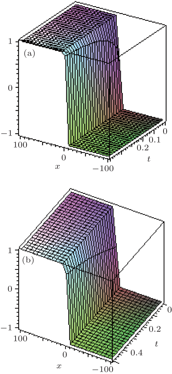
Fig. 6. The exact solution for Eq. (95) with α = 0.5 (a) and α = 1 (b) respectively, when k = 1, c = 1, w = 2, y = 0, and l = 1.
5. Conclusion
In this paper, we have derived bright and dark soliton solutions of three nonlinear partial differential equations with fractional order. As a result, some new exact soliton solutions for them have been successfully obtained. The ansatz method was effectively used to achieve the goal set for this work. The conditions of existence of solitons are presented. The proposed method permits us to obtain in a direct manner exact bright and dark soliton solutions for the fractional differential equations under consideration. We have predicted that fractional complex transform can be extended to solve many systems of nonlinear fractional partial differential equations in mathematical and physical sciences by ansatz method.


 , Bekir Ahmet2, ‡,