Terahertz (THz) wave has attracted extensive attention in many scientific applications including detection, communication, biomedicine, imaging, and spectroscopy.^[1–7] One of the important applications that have been continuously accelerating the development of the THz gyrotron is sensitivity-enhanced nuclear magnetic resonance (NMR) via dynamic nuclear polarization (DNP).^[5,7] The required level of the output power and the needed specific spectral characteristics make the gyrotron oscillator a most promising and high-performance device for such an application. The gyrotron is a fast-wave vacuum electron device based on the mechanism of electron cyclotron maser (ECM) and can operate with an over-mode open cavity, which permits a considerably higher output power level than the semiconductor device and other competing THz vacuum sources, such as the extended interaction oscillator (EIO), the extended interaction klystron (EIK) and the backward-wave oscillator (BWO).^[6] Compared with the free electronic laser (FEL), the gyrotron also has the advantage in compact size.

The operating frequency of a gyrotron is close to the electron cyclotron frequency, ω_c = eB₀/γm₀, where B₀ is magnetic field and γ is relativistic factor, e and m₀ are electron charge and mass, respectively. For a gyrotron operating at the sth cyclotron harmonic, its operating frequency can be estimated to be f = 28sB₀/γ. So one can see that a very strong magnetic field is required when the gyrotron operates at THz band in the fundamental mode, but the magnetic field can be significantly reduced when the gyrotron operates at a harmonic of electron cyclotron resonance.^[6,8,9] Though quite a lot of relevant researches have been carried out,^[10–16] the dynamics of axial mode behavior which plays an important role in determining the performance of tunable gyrotrons, is still rarely studied.

A traditional gyrotron, such as the gyrotron used in the fusion plasma heating, usually adopts an interaction circuit, which operates in the fundamental axial mode with a high quality factor and radiates almost at a single frequency. However, the gyrotron for DNP-NMR application needs a reasonable tunable bandwidth to well achieve the synchronization between the THz wave and the NMR polarization system. The successful solution to realize frequency tunable gyrotron is to tune the system parameters to force the system to transit between different axial modes with comparatively low quality factors in the open-cavity interaction circuit. Hence, systematic studies of dynamics of the axial mode transition in open cavity are very important to promote the development of the frequency tunable THz gyrotron.

Many previous studies of mode startup process have assumed a fixed field profile,^[17–20] but this assumption is not well fulfilled in DNP-NMR gyrotron which operates based on axial mode transition. Hence, the non-fixed field time-dependent code based on the time-domain nonlinear theory is developed and used to study the performance of the 0.33-THz gyrotron oscillator which operates at the second-harmonic cyclotron and low voltages. Then a new interaction mechanism about propagating waves, featured by wave competition and wave cooperation, is presented and provides a new insight into the beam-wave interaction to study the dynamic axial mode behavior. What is more, some non-stationary phenomena in the mode startup process which cannot be observed under the fixed field assumption are found and analyzed.

The counter-rotating TE_−3,4 cylindrical waveguide mode is selected as an operating mode because this mode can provides strong coupling with the beam among second-harmonic modes while the guiding center of electron beam is far enough from the center of cavity. The points of highest intensity (the first Bessel function maxima) of the mode pattern are away from the cavity walls, thereby avoiding the high ohmic heating encountered with the whispering gallery modes (m ≫ n for mode TE_m,n) and the mode competition with high-order TE_0,n modes. Moreover, this mode is comparatively isolated from other surrounding competing modes in the beam-wave interaction spectrum.

The excitation frequency of a gyrotron is determined by the frequency of eigenmode in the interaction cavity. It is always close to the cutoff frequency f_m,n of the cavity. For the TE modes in the vacuum cylindrical waveguide, the cutoff frequency is

For operation at 0.33 THz in the mode TE_−3,4, the cavity radius (radius of the straight section) is chosen to be 2.109 mm. The geometry of the gyrotron circuit is shown in Fig. 1. A conventional cylindrical waveguide cavity^[21,22] is adopted and consists of one uniform and three tapered waveguide sections. The angles are θ₁ = 3°, θ₂ = 0.7°, and θ₃ = 2.1° respectively. The lengths of the sections are L₁ = 7.5 mm, L₂ = 35.5 mm, L₃ = 21.5 mm, and L₄ = 23 mm respectively. A long cavity with a middle section length L₂ of about 39λ, where λ is the free-space wave length, is chosen to reduce the starting current^[23] of the operating mode and make the excitation of high-order axial modes (HOAMs) easier, thereby enhancing the frequency tuning ability.

Fig. 1.

	Figure Option ViewDownloadNew Window
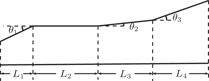
	Fig. 1. Geometry of the 0.33-THz gyrotron circuit consisting of four sections.

The guiding center radius of electron beam r_c is selected to be 0.93 mm, where the first maximum of Bessel function J_m+n(x) is located, to obtain favorable coupling to the operating mode. The coupling factor C_m,n between electron beam and operating mode is given by^[23]

Cold cavity simulation allows one to determine cavity parameters efficiently, such as the resonant frequency of the cavity eigenmodes, axial field profile and quality factor Q, which can be conducible to the cavity design. The characteristic of the cold cavity is analyzed based on the weakly irregular waveguide theory.^[24] In the cold cavity without electron beam, a series of resonant axial modes exist which can be specified by their resonant frequencies and axial profiles. The simulation results give the values of resonant frequency and the diffractive quality factor Q_d of operation mode TE_−3,4,q ranging from q = 1 to q = 7, which are listed in Table 1, where q is the axial mode number. The diffractive quality factor is related to the axial index by the law.^[25]

Table 1.

Table 1.

Table 1. Frequencies and diffractive quality factors for the TE−3,4,q modes. . q Cold resonant frequency/GHz Qd 1 330.01 88034 2 330.08 21992 3 330.20 9751 4 330.37 5455 5 330.59 3463 6 330.86 2398 7 331.18 1784

Table 1. Frequencies and diffractive quality factors for the TE−3,4,q modes. .

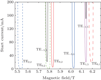
Mode competition can be studied based on the starting current preliminarily. The starting current is the threshold to be overcome to excite a given wave guide mode and can be calculated from the linear theory of the gyrotron oscillator.^{[21,23,26,27]} Based on the cold cavity analysis above, starting currents for the operating and neighboring modes are shown in Fig. 2. It reveals that in a magnetic field range of 6.0 T–6.1 T, the operation mode TE_−3,4 is comparatively isolated from other surrounding competing modes.

Fig. 2.

	Figure Option ViewDownloadNew Window
	Fig. 2. Starting oscillation currents of cavity modes near the operating mode TE−3,4,1 as a function of magnetic field, where dashed lines represent fundamental-harmonic modes while solid lines refer to second-harmonic modes with beam parameters: Vb = 12 kV and α = 1.75.

For analyzing the beam-wave interaction, time-domain self-consistent calculations are employed by using the following theoretical model. A thin annular electron beam is located at the r_c radius (as shown in Fig. 3), with the thickness and velocity spread ignored. The electrons follow helical trajectories in static magnetic field B₀ and interact with the operation TE mode.

Fig. 3.

	Figure Option ViewDownloadNew Window
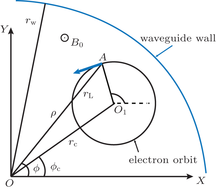
	Fig. 3. Electron orbit in the waveguide.

The transverse electric field of the mode is expressed as

According to the well-known Maxwell equations, we neglect the space charge effect and obtain the wave equation

Neglecting the beam effects on the transverse mode profile, we operate on both sides of Eq. (5) with

The transverse alternating beam current density J_t can be expressed as^[28]

Here I_b is the beam current, W_j is a normalized weighting factor for the j-th electron, υ_zj and υ_tj are the axial velocity and the transverse velocity of the j-th electron, respectively.

Substitute Eq. (8) into Eq. (7) and express the field in the guiding center O₁, then we will obtain

The phase factor is Λ_j = − ωt_j + (m − s)ϕ_c + sθ_j, and the radiation boundary conditions^[28] are

The electron beam is represented as an ensemble of particles in the form of function (8) and their trajectories are traced. Their orbits in the interaction region can be described by the relativistic equation of motion

Here p is the electron momentum, v is the velocity of the electron, E and B are the mode electric and magnetic fields respectively, and B₀ is the external static magnetic field.

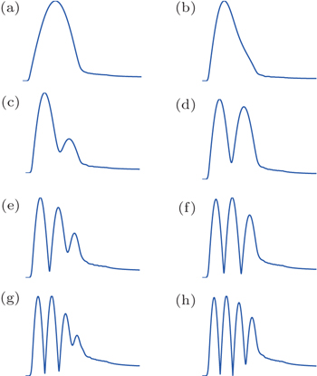
The beam-wave interaction theory consists of the system of Eqs. (9) and (11) which describe self-consistently both the dynamics of the electrons and the excitation of the electromagnetic field.^[29,30] Based on the time-domain self-consistent nonlinear theory, a simulation code is developed.

In Fig. 4, the axial field structures show the continuous transition from low-order axial modes (LOAMs) to HOAMs and provide a mechanism for the continuous frequency tuning. Their frequencies and field profiles are close to those in the previous cold cavity analysis. The non-fixed self-consistent field structure in the mode transition process can be decomposed into a forward wave and a backward wave. The mode axial profile is described as

Fig. 4.

	Figure Option ViewDownloadNew Window
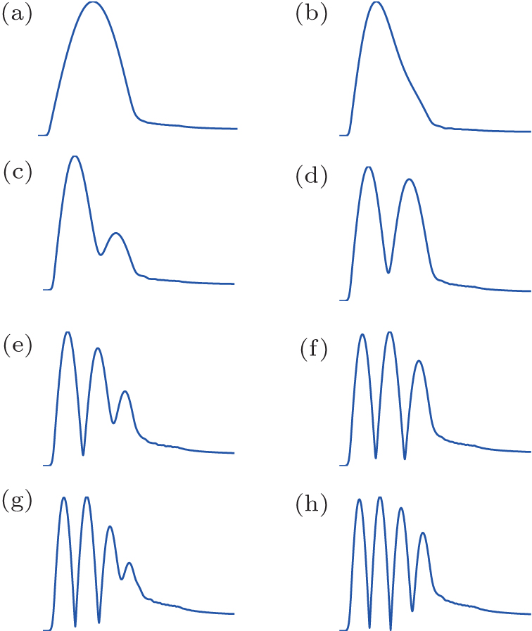
	Fig. 4. Transitions of self-consistent axial field profiles for axial modes from q = 1 to q = 4.

Figure 5 shows the power components of the first axial modes under three different operation magnetic fields. In Fig. 5(a), for a lower magnetic field condition B₀ = 6.022 T, the forward wave starts from the cut-off section (L₁ in Fig. 1 corresponds to 0 mm–7.5 mm) end, grows up in the downstream direction and reaches its maximum at the midpoint of the cavity. Then it diminishes until it propagates out of the cavity and travels with a constant amplitude. On the other hand, the backward wave starts from the cavity end, propagates with an almost one half amplitude of the forward wave, and suddenly vanishes at the cut-off section end. In other words, wave is cutoff in the cut-off section and behaves like a standing wave in the cavity where the main energy exchange happens. Then it transforms into a travelling wave in the up tapered sections (L₃ and L₄ in Fig. 1 correspond to 43 mm–87.5 mm) without energy extraction from electron beam. With magnetic field increasing to 6.03 T in Fig. 5(b), the backward wave extracts more energy from electron beam and is enhanced, and then it reaches a maximal value comparable to the forward wave does. The forward wave profile remains the same as that in Fig. 5(a) except that the profile peak slightly moves downstream.

Fig. 5.

	Figure Option ViewDownloadNew Window
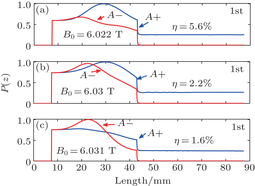
	Fig. 5. Normalized power profiles of the first axial mode under different magnetic fields: (a) B0 = 6.022 T, (b) B0 = 6.03 T, and (c) B0 = 6.031 T.

Under a higher magnetic field B₀ = 6.031 T in Fig. 5(c), the forward wave decreases and its profile in the cavity becomes flat which indicates that the forward wave starts to be suppressed by the backward wave. The backward wave interacts first with the electron beam in the left of cavity and extracts energy ahead of the forward wave, which gives rise to the energy and velocity spread of the electrons. So the forward wave cannot efficiently interact with the beam and results in a lower efficiency as shown in Fig. 5. This situation becomes more serious in the Fig. 6(b) with B₀ = 6.038 T, the forward wave profile is sunken in the cavity and the backward wave interacts with the beam primarily. The wave decomposition has provided an insight into the beam-wave interaction, and the transition from forward wave interaction to backward wave interaction happens in the LOAM operation area. It is concluded that there is a competition between the forward wave and the backward wave, and the two-wave competition leads to the decline in efficiency with increasing the magnetic field.

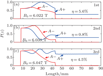
Furthermore, it is interesting that under the magnetic field B₀ = 6.047 T in Fig. 6(c), where the HOAM TE_−3,4,3 operates, the forward wave does not continue to diminish as that shown in Fig. 5, and by contraries it grows up and propagates gently with three slight fluctuations. Its amplitude remains almost at the same level comparable to the peak of the backward wave. The backward wave profile remains unchanged except that the profile peak slightly moves upstream. This dramatical phenomenon can be explained by the fact that when the backward wave propagates in the upstream direction, it cannot travel out through the left port because the operating frequency is lower than the cutoff frequency of the left port cross section. So the backward wave is reflected back and the wave power is converted into the power of the forward wave. The effective electron transit angle is defined as Θ_eff = (ω − k_zv_z − sΩ₀)τ, where ω is the wave angular frequency and τ is the electron transit time. It is the wave phase variation observed by the electron in traversing the interaction space. The mismatch between the effective electron transit angles of the backward wave and the forward wave is 2k_zv_zτ. In the LOAMs operation, the operation frequency is close to the cut-off frequency in the middle section (L₂ in Fig. 1) of the cavity and their effective transit angles are close to each other, indicating that the intensities of two waves each coupling with the electron beam are comparable to each other. So an obvious wave competition is observed. On the other hand, an HOAM corresponds to a greater propagation constant k_z, and the mismatch of the effective electron transit angles becomes larger. The intensities of two waves each coupling with the electron beam cannot be maintained at the same level. The forward wave obtains a weak coupling with the electron beam and becomes seriously detuning from resonance. So the power profile of the forward wave exhibits three slight fluctuations in Fig. 6(c), indicating no competition with the backward wave. It is concluded that comparing with the two-wave competition in the LOAM operation area, the beam-wave interaction in the HOAM operation area behaves as two-wave cooperation.

Fig. 6.

	Figure Option ViewDownloadNew Window
	Fig. 6. Normalized power profiles of the axial modes from q = 1 to q = 3 under different magnetic fields: (a) B0 = 6.022 T, (b) B0 = 6.038 T, and (c) B0 = 6.047 T.

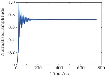
In the time-dependent simulation some non-stationary phenomena are observed. Under the magnetic field 6.038 T where a LOAM operates, non-stationary oscillation is observed at a saturation amplitude level. As shown in Fig. 7, in the first 27 ns the amplitude at the output port rises to a global maximum value. The field profile at 27 ns is shown in Fig. 8, which is the typical field profile of the TE_−3,4,2 mode. Then there is a following damped oscillation of about 200 ns with a non-stationary time-dependent field profile, and figure 8 also shows a different field profile at 32.5 ns in black dashed line. The periods of these oscillations are all about 10 ns, which corresponds to a 0.1 GHz auto modulation frequency. This low-frequency modulation can be attributed to the mode competition between the first and second axial mode. The cold resonant frequencies of the first and second axial modes are 330.01 GHz and 330.08 GHz, respectively. The difference between their frequencies is about 0.07 GHz and is close to the 0.1-GHz beating frequency observed in the simulation. The discrepancy between 0.07 GHz and 0.1 GHz results from the frequency pulling effect. So the axial mode competition leads to the following long-time damped oscillation and is considered as another reason for the decline in output efficiency.

Fig. 7.

	Figure Option ViewDownloadNew Window
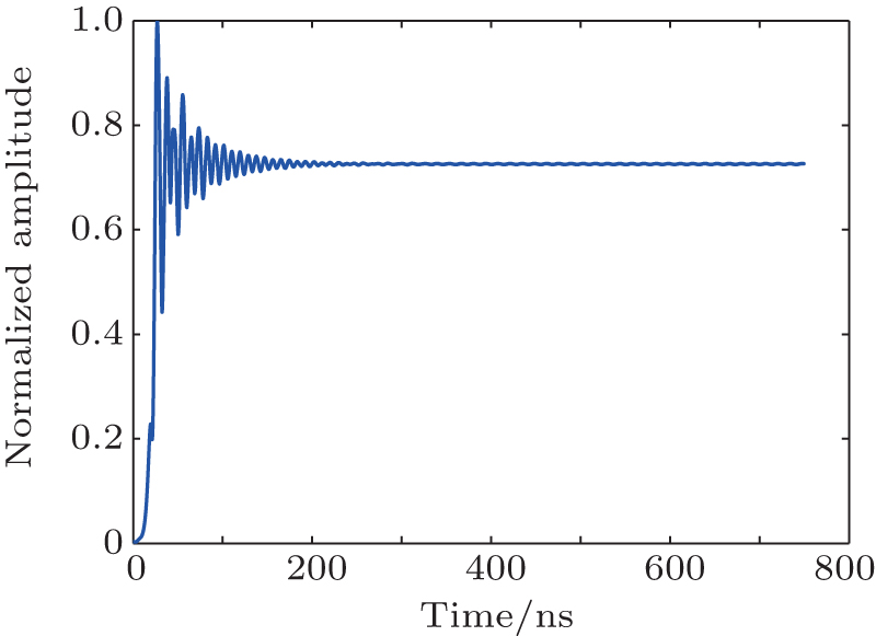
	Fig. 7. Time evolution of the output amplitude under a low magnetic field.

Fig. 8.

	Figure Option ViewDownloadNew Window
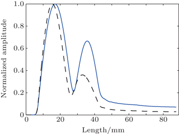
	Fig. 8. Profiles of normalized filed versus length at 27 ns (blue solid line) and 32.5 ns (black dashed line).

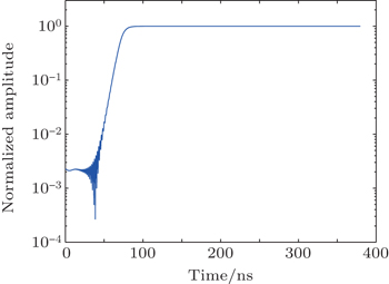
Unlike the startup scenarios in Fig. 7, the temporal growth of the filed amplitude at the output port under a high magnetic field 6.063 T is shown in Fig. 9. Oscillation at a low-amplitude level is observed. The field profile and amplitude change rapidly until HOAM TE_−3,4,5 mode dominates at 45 ns, and the field profile remains nearly unchanged afterwards. Then no instability is observed and the field grows up fast, exponentially. Finally it reaches a steady state at 80 ns. The corresponding frequency spectrum is shown in Fig. 10 and the frequency of the peak point is 330.59 GHz with no sideband.

Fig. 9.

	Figure Option ViewDownloadNew Window
	Fig. 9. Time evolution of the output amplitude under a high magnetic field.

Fig. 10.

	Figure Option ViewDownloadNew Window
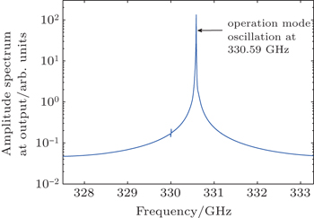
	Fig. 10. RF spectrum at the geometry output.

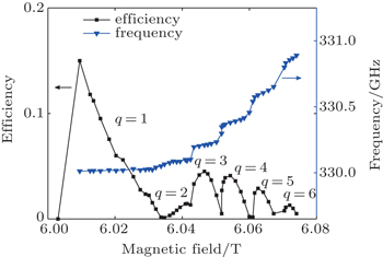
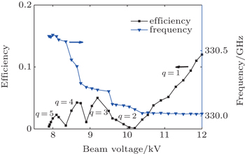
The output efficiency and frequency tuning range via magnetic field and beam voltage tuning are shown in Figs. 11 and 12, respectively. In Fig. 11 six axial modes could be excited in a frequency tuning range from 329.92 GHz to 330.73 GHz. The highest efficiency is obtained in the interaction with the first axial mode (q = 1) and the interaction switches to HOAMs when increasing the magnetic field. In Fig. 12, five axial modes could be excited with tuning frequency in a range from 330.09 GHz to 330.62 GHz. Both the power and frequency curves demonstrate obvious axial mode transition processes, and the envelopes of the power curves are qualitatively consistent with other similar experimental results,^[31] which indicates the reliability of the theoretical analysis. The synchronization condition for the beam-wave interaction can be described as ω ≈ k_zv_z + sΩ₀. Increasing the magnetic field or reducing the beam voltage increases the relativistic cyclotron angular frequency, and the wave angular frequency is increases up until the synchronization condition is met self-consistently. Corresponding axial modes are excited one after another and continuous frequency tuning with the axial mode transition is realized, leading to similar spectra of output efficiency shown in Figs. 11 and 12.

Fig. 11.

	Figure Option ViewDownloadNew Window
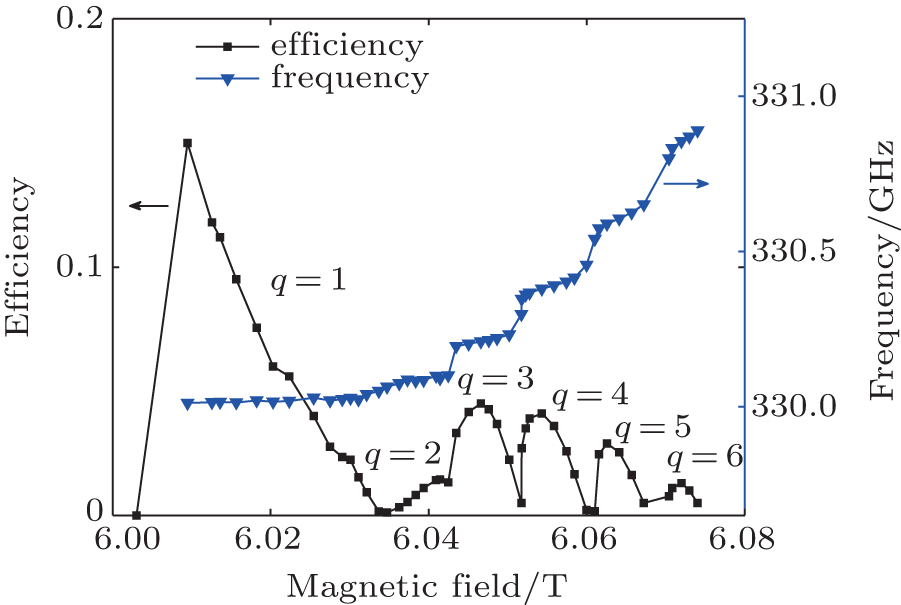
	Fig. 11. Self-consistent simulations of efficiency and frequency tuning as a function of magnetic field.

Fig. 12.

	Figure Option ViewDownloadNew Window
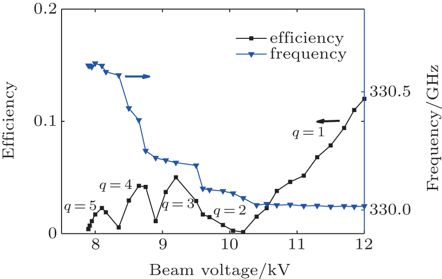
	Fig. 12. Efficiency and frequency tuning as a function of beam voltage.

Generally speaking, a compromise between the smooth efficiency output and the tuning bandwidth determines the overall performance of the device, which leads to a finite-bandwidth. The HOAMs have lower quality factors than the LOAMs and exhibit weaker coupling with the electron beam. Utilizing a long cavity or increasing the beam current makes the HOAMs excitation easier to provide wider frequency tuning bandwidth, but the problem of mode competition from both axial modes and transverse modes can be critical. In our investigation, the long cavity increases the Q factors of HOAMs and enhances the wave feedback. But on the other hand, the high Q factor leads to a large Q factor separation (Q-separation) between neighboring axial modes, and the Q-separation between the q-th axial mode and (q + 1)-th axial mode can be estimated as (2q + 1)Q₁/q²(q + 1)², where Q₁ refers to the Q factor of the fundamental axial mode. The large Q-separation produces a negative effect on the transition process between neighboring axial modes and results in an axial-mode competition. As shown in Fig. 11, the crater in the output efficiency spectra, which is located in the transition area between the fundamental axial mode and the second axial mode, results from the mode competition between the two axial modes in the transition process shown in Fig. 7. In the HOAM area, the output efficiency exhibits obvious fluctuations, which are closely related to the axial mode transition. Increasing the beam current is another way to excite HOAMs, but like the situation above, an axial-mode competition can be excited and more seriously a non-stationary oscillation is possible. When the current exceeds the threshold of competition modes, transverse mode competition can also be induced. So it should be always notable to avoid mode competition from both axial modes and transverse modes, which would deteriorate the stability of the device operation.

In this paper, the non-fixed field time-dependent code is developed and used to investigate the output performance of the second harmonic gyrotron oscillator. A frequency tuning range of 0.85 GHz with an efficiency range of 0.12%–15% is achieved by tuning magnetic field. By tuning voltage, a frequency tuning range of 0.6 GHz with an efficiency range of 0.14%–12% is achieved. Both efficiency spectra exhibit obvious fluctuations in the HAOMs area with an average efficiency of about 2%. The characteristics of the axial mode transition are analyzed, and some new non-stationary phenomena in the mode startup process which cannot be observed under the fixed field assumption are found.

Results show that the transition from forward wave interaction to backward wave interaction happens with magnetic field increasing. Fundamental axial mode interaction can provide higher peak output efficiency but the two-wave competition leads to the rapid decline in output efficiency with magnetic field increasing. The interaction in the HOAM area behaves as two-wave cooperation and can provide better frequency tunability with comparatively low efficiency. What is more, mode competition between the first and second axial mode is found under the low magnetic field and this is considered as another reason for the decline in output efficiency. The problems from both axial modes and transverse modes should always be notable, and the mode competition should be avoided to achieve stable operation. Generally speaking, the compromise between the stable, smooth output and the tuning bandwidth determines the overall performance of the device.

The present work should be beneficial to the gyrotron used in DNP-NMR and other terahertz applications, in which the gyrotron needs a reasonable tunable bandwidth and operates based on axial modes transition.